Charts of Atmospheric CO2, Carbon Isotopes, Oxygen and Methane

 I started making charts of atmospheric CO2 in 2009, when the global average CO2 concentration was 386 ppm.  I updated my charts in 2012, at 392 ppm, and in 2017, at 405 ppm, and at the end of 2021, at 418 ppm. 

The monitoring stations are located from the far north, at 82° N in Canada to the South Pole.  Scripps Institute has managed most of these stations since the 1950s, first under the direction of Charles Keeling, and later under his son, Ralph Keeling.  I also included records from a few obsolete legacy stations that were operated by foreign governments.  I standardized my chart displays using cool colors to represent the Northern Hemisphere, and warm colors for the Southern Hemisphere.

The amplitude of the CO2 seasonal cycle varies with latitude, from high amplitude in far northern latitudes to very little amplitude at the South Pole.  The seasonal cycle is driven by seasonal plant growth and decay on lands with temperate climate, which are concentrated in the Northern Hemisphere.  Agriculture, which is also concentrated in the Northern Hemisphere, also contributes to the seasonal cycle.  I took advantage of this for my standard display, overlaying low amplitude over higher amplitude traces, so that all traces can be seen.

In general, CO2 concentration in the atmosphere is growing exponentially, a fact noted by Isaac Asimov in 1959.  In 2009, I made an exponential function, beginning at the pre-industrial CO2 concentration of 280 ppm in 1800, with an eyeball-fit to the data from 1957 to 2009.  Here’s the function, and the chart beginning in 1800, updated with CO2 data through 2021.  This chart has the “hockey stick” impression that characterizes many climate-change charts.

CO₂ concentration, ppm = e^(n*0.001854) + 280, where n = the number of months since Jan. 1800

This function would predict that global CO2 would pass 450 ppm in January, 2032 (ten years from now), and pass 500 ppm in August, 2043.

The exponential function seems to be slightly overstating the rate of CO2 growth since 2009, so I tried an alternate formula for the forecast in coming decades, a second-degree polynomial with a least-squares fit to the global average CO2 from 1974 to 2009.  That formula is CO2 in ppm = 0.000104*x²+0.0897*x+331.66, where x is the number of months from July, 1974.  This formula predicts global CO2 will pass 450 ppm in June, 2034, and pass 500 ppm in July, 2050. 

Certainly, these forecasts are simple extrapolations, and include none of the analysis of policies and economics which should be the basis of forecasting.  But it’s worth noting that my exponential forecast from 13 years ago is pretty much right on the money, overshooting by only one or two parts per million.  The last thirteen years has seen unprecedented growth in renewable energy technologies, but so far without significant impact on the rate of CO2 growth.  Here are the two forecasts on the same chart.

The seasonal cycle can easily be filtered from the data, leaving the long-term trend at each station.  From this, it’s easy to see that the Northern Hemisphere leads the Southern Hemisphere in rising CO2.  About 90% of fossil fuel burning happens in the Northern Hemisphere, and CO2 accumulates in the far north, while dispersing to the south. 

The difference in concentration from the far north to the South Pole has been increasing as larger volumes of fossil fuels are burned each year, from about 3 ppm in the 1980s to over 5 ppm now.  The chart below shows the difference in the one-year time-averaged CO2 concentration measured in Alert, Canada, at latitude 82° North, and the South Pole. 

The amplitude of the seasonal cycle has also been increasing in the far north.  The amplitude of the cycle increased from 15 ppm to 20 ppm since the mid-1970s.  This probably reflects increased agriculture and farm productivity in the Northern Hemisphere as world population has doubled.  Previous work showed that seasonal fossil-fuel use is volumetrically inadequate to produce the change in the atmospheric CO2 seasonal cycle.  https://dougrobbins.blogspot.com/2012/04/modeling-global-co2-cycles.html

Carbon comes in two common naturally occurring isotopes, C¹² and C¹³.  Various processes, including life processes, sort the isotopes, favoring the accumulation of one or the other isotope.  Photosynthesis favors C¹², so everything with carbon derived from plants, including lumber, your mashed potatoes, you, me, and fossil fuels is enriched in C¹².  Scientists use a measure of the C¹³/C¹² ratio written as d¹³C , and called delC13.  As fossil fuels are burned the C¹²-enriched carbon in CO2 changes the ratio of these isotopes in the atmosphere, lowering the value of delC13.  DelC13 continued to fall from 2009 to 2021, reflecting a growing fraction of carbon from fossil fuels in the atmosphere. 

Carbon isotopes in the atmosphere are also affected by the seasonal cycle of plant growth on the temperate land mass of the Northern Hemisphere.  As plants grow during the northern summer, the lighter isotope C¹² is preferentially removed from the atmosphere, and returned during the winter months as plants decay.

After filtering the seasonal cycle, we see that the Northern Hemisphere leads the Southern Hemisphere in falling DelC13.  As an aside, the residual fluctuations in the trend have a strong correlation to the Oceanic Nino Index (ONI), reflecting sea surface temperatures in the Pacific.  https://dougrobbins.blogspot.com/2013/11/carbon-isotopes-in-atmosphere-part-ii.html

Interestingly, if all of the carbon released by fossil fuels stayed in the air, the DelC13 value would be much lower, about -13, instead of -8.5.  The measured dilution of carbon with the isotope signature of fossil fuels provides a way of estimating the volume of all carbon reservoirs exchanging carbon with the atmosphere.  Currently, the reservoirs freely exchanging carbon with the atmosphere have a carbon mass of about 5200 gigatonnes, before accounting for additional carbon in the system from new burning of fossil fuels.  That’s about 6 times the mass of carbon currently in the atmosphere.  https://dougrobbins.blogspot.com/2013/11/how-big-is-carbonsphere.html

Atmospheric oxygen is also influenced by burning of fossil fuels.  Oxygen is consumed, causing atmospheric O2 to fall.  The atmosphere is about 21% oxygen, and the decline is only about 0.08%, so there is no threat to breathing.  Still, the decline can be measured precisely.  The decline in oxygen is reported in units per meg, which is equivalent to ppm in this range of values.

After filtering the seasonal cycle, we see that the Northern Hemisphere leads the Southern Hemisphere in oxygen decline, because most fossil fuels are burned in the Northern Hemisphere.  The total volume of oxygen decline is very close to the expected consumption of oxygen considering the reported volumes of fossil fuels burned and deforestation, as reported in this previous post.  https://dougrobbins.blogspot.com/2019/12/understanding-source-of-rising.html

Atmospheric methane (C4) is also increasing as a result of human emissions.  Methane is a much more powerful greenhouse gas than CO2, but has a shorter lifespan.  CO2 has a half-life of 120 years, while methane has a half-life of about 10 years.  This is why the climate scientists use the parameter GWP (global warming potential) to represent the different strength of various greenhouse gases over an effective time frame.  The GWP of CO2 equals 1, by definition, for all time intervals.  For methane, the warming potential over 20 years (GWP-20) is 84 – 87, and over 100 years is 28 – 36.  Over shorter intervals, methane is an even stronger greenhouse gas.  Currently, methane concentration in the atmosphere is about 1.9 ppm (i.e. 1900 ppb).  In absolute terms, methane warmed the earth by about 0.52 W/m2, compared to 2.11 W/m2 for CO2, for the latest year reported by NOAA, 2020.  All other greenhouse gases combined contributed another 0.55 W/m2.  Methane also has a seasonal cycle in both hemispheres with high values in the summer and low values in the winter, but I don’t know the explanation for the seasonal cycle. 

As the concentrations of CO2 and methane in the air rise, the atmosphere will absorb heat at a faster rate, leading to destructive climate change.  Temperatures and climate change will not stabilize until carbon emissions reach zero.  I will update my charts on carbon emissions when summary data for 2021 is released in the BP Statistical Summary of World Energy in July.  Apart from a small pandemic-related decline in emissions in 2020, the world continues to add CO2 to the atmosphere at an ever-increasing rate.  If the world had acted to reduce emissions three decades ago, simply reducing emissions might have been a reasonable policy.  However, in our current situation, outright elimination of carbon emissions is required to avoid some level of catastrophic consequences. 

Globally, we need to reduce emissions to 50% by 2035, and to zero some time between 2050 and 2070.  I am very pessimistic that we have the public understanding or political will to reach these goals.  As Bill Gates wrote in 2021, "To avoid a climate disaster, we have to get to zero greenhouse gas emissions….The case for zero was, and is, rock solid.  Setting a goal to only reduce our emissions—but not eliminate them—won’t do it.  The only sensible goal is zero.”

References:

CO2, CO2 carbon isotopes, oxygen and methane data, including obsolete CO2 stations

https://scrippsco2.ucsd.edu/data/atmospheric_co2/sampling_stations.html

https://scrippso2.ucsd.edu/data.html

https://gml.noaa.gov/dv/data/

https://data.ess-dive.lbl.gov/view/doi:10.3334/CDIAC/ATG.015

https://www.osti.gov/dataexplorer/biblio/dataset/1409297

https://carbonmapper.org/data/

Isaac Asimov, "No More Ice Ages?" prediction and commentary on global warming,
in Fantasy and Science Fiction, Jan. 1959, republished in Fact & Fancy, 1962 and Asimov on Chemistry, 1974. 

Global Warming Potential

https://www.epa.gov/ghgemissions/understanding-global-warming-potentials#:~:text=Methane%20(CH4)%20is%20estimated,uses%20a%20different%20value.).

GWP-20 for methane = 84 to 87; GWP-100 for methane = 28 to 36 (also reported as 25)

Radiative Forcing for various greenhouse gases

https://gml.noaa.gov/aggi/aggi.html

Global Heat Budget #1: Anthropogenic Heat

I have been away from my blogs for far too long.  I will try to post a series on the global heat budget.

Previously, I posted a lot of work on atmospheric CO2, considering the geographic distribution, isotope data, rates of change, comparison to man-made emissions from various sources, and interaction of the atmosphere with global carbon reservoirs.  The latest summary post is here:

http://dougrobbins.blogspot.com/2016/08/the-keeling-curve-and-global-co2.html

I deliberately avoided the question of climate change to focus on the science of atmospheric CO2.

For the past year, I’ve been studying on the problem of global warming (the first-order consequence of greenhouse gases) and climate change (the higher-order consequences of greenhouse gases).  And I’ve been posting less while I worked to understand the data.

I’m going to present what I’ve learned as a series of short posts, rather than writing a book.

The very short version is this:

The Global Heat Budget; The Very Short Version

People have raised the concentration of atmospheric CO2 by burning fossil fuels.  The volume of CO2 released by fossil fuels has increased sharply since about 1950, and continues to increase today.

CO2 and other greenhouse gases retain heat in the atmosphere.  The quantity of heat is easily calculated as a function of the concentration of CO2 in the air.  We can calculate the amount of heat that has been trapped to date, and we can forecast the heat that will be trapped in the future.

Heat is increasing in heat sinks on earth.  Observations show that the amount of heat appearing in earth’s heat sinks is approximately equal to the heat retained by greenhouse gases.  The heat is showing up as rising ocean temperatures, melting ice, and a warmer atmosphere.  The quantity of heat appearing in these systems has been measured by high-accuracy monitoring programs since about 2003.  The warming ocean accounts for about 95 percent of our estimates of anthropogenic heat.  Retained heat due to greenhouse gases is the only credible source for the heat appearing in heat sinks.

Sea-level is rising.  Sea level rise has been documented by tidal gauges for 130 years, and by high-accuracy satellite measurements since 1992.  The amount of sea level rise matches the observed volumes of melted ice, thermal expansion of the ocean, and ground-water extraction.  The fact of rising sea level confirms observations of melting ice and warming oceans.

Higher atmospheric CO2 concentrations are inevitable for the foreseeable future.  Quantitative forecasts of future heating indicate serious and expensive problems will develop for the nation & the world.

Atmospheric CO2 has risen as a consequence of fossil fuel emissions.  The following chart is my version of the Keeling Curve (http://dougrobbins.blogspot.com/2016/08/the-keeling-curve-and-global-co2.html) showing global CO2 concentration, including high-amplitude seasonal cycles in the Northern Hemisphere, and low-amplitude seasonal cycles in the Southern Hemisphere.

History of Study of CO2 as a Greenhouse Gas

The physics of CO2 as a greenhouse gas is settled science, based on published studies dating back over 150 years.  High accuracy programs to measure melting ice, ocean temperatures, and rising sea level have been in place in recent decades, long enough to yield conclusive results.

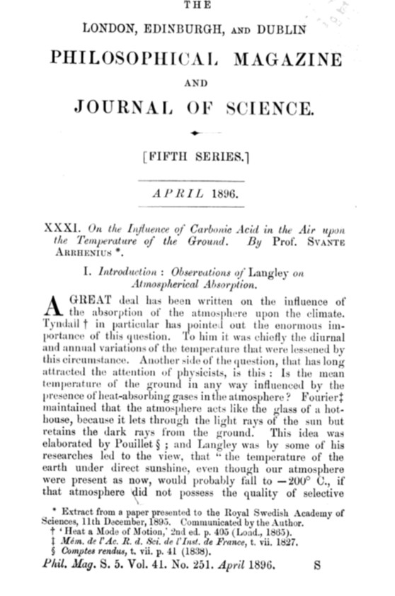
Carbon dioxide was first proved to be a greenhouse gas by John Tyndall in 1859, proving speculation that began in 1820.  The planet-wide effect of changing CO2 concentrations was calculated by the Swedish chemist Arrhenius and published in 1896.  Arrhenius was originally attempting to find the cause of the ice ages, but later recognized the possibility that fossil fuel emissions could change the climate, and published that result in 1906.  Quantitative measurements of CO2 and rising temperatures were published in 1938 by Guy Callendar.  Systematic global measurements of CO2 concentrations began in 1955 by Charles Keeling.  Satellite measurements of sea level rise began in 1992.  Satellite measurements of Antarctic and Greenland ice mass began in 2003.  Detailed, comprehensive and continuous measurements of ocean temperatures began in 2004.

Calculation of Heat Retained by Greenhouse Gases

Greenhouse gases are mostly transparent to wavelengths of visible light, which carry most of the energy from our sun.  Visible light strikes the earth and is converted to heat.  Normally, some portion of that energy is re-radiated into space as thermal infrared radiation.  But greenhouse gases are opaque to infrared wavelengths, and trap heat in the atmosphere as a function of the concentration of those gases.  As greenhouse gases have accumulated in the atmosphere, lower levels of the atmosphere have warmed.  Higher levels of the atmosphere have cooled, as more heat has been trapped near the surface.

NOAA publishes historical tables of the atmospheric heating coefficients (known by the awkward and uninformative phrase *radiative forcing*) for anthropogenic greenhouse gases, dating back to 1979.  The coefficients are prepared according to international standards, taking into account cloudiness and angle of solar incidence to yield a global average.  You can do the math yourself to calculate annual heat retained by each greenhouse gas, which I have done.  Carbon dioxide represents about two-thirds of the heat retained in the atmosphere by greenhouse gases.  Methane, nitrogen oxide, chlorofluorocarbons (CFCs) and minor greenhouse gases account for the rest of the heat retained by greenhouse gases. 

https://www.esrl.noaa.gov/gmd/aggi/aggi.html

In 1979, greenhouse gases retained about 7 x 10²¹ joules.  By 2016, greenhouse gases retained about 1.2 x 10²² joules, an increase of 78% in annual heating.  It’s difficult to conceptualize how much heat is represented by 10²² joules.  A joule is about ¼ of a standard calorie – the heat required to raise a gram of water by one degree C.  It’s a small amount of heat.  But 12,000,000,000,000,000,000,000 joules is a lot of heat.  Later in this series, we’ll consider how the earth can absorb that quantity of heat, and where the heat is going.

Aerosols and Anthropogenic Cooling

Aerosols are the least-well quantified anthropogenic influence on earth’s climate.  Sulfate aerosols cool the atmosphere by making clouds more abundant and reflective.  Sulfates can originate from volcanic eruptions, but are also a common industrial pollutant.  Carbon black aerosols warm the atmosphere by absorbing sunlight. 

Sulfate emissions have dropped dramatically in the United States and Europe over the past 25 years, thanks to regulations intended to limit acid rain, but world-wide sulfate emissions have continued to grow.  The average global impact of sulfates and black carbon aerosols is shown in the following graphs, but the more significant impacts are regional.  South Asia suffers from the greatest carbon black emissions and impact, while China is now the source of most sulfate emissions.

IPCC Net Anthropogenic Heating and Cooling

The IPCC (International Panel on Climate Change) 5th Climate Assessment contains a table of anthropogenic heating and cooling coefficients.  The IPCC numbers for conventional greenhouse gases are identical to NOAA, but IPCC also recognizes other anthropogenic factors, which can both heat and cool the atmosphere.  These factors act by direct absorption of sunlight, or by a greenhouse effect that is restricted to certain levels in the atmosphere.  The IPCC recognizes the warming factors of tropospheric ozone (O3), stratospheric water vapor (H2O), black carbon on snow, and contrails.   IPCC recognizes cooling factors, including land-use changes (which affect the reflectivity of the earth), stratospheric ozone, and aerosols. 

Here is a chart based on IPCC data, showing anthropogenic heating and cooling coefficients (*radiative forcing*).

Primary Anthropogenic and Other Heat

Strangely, to me, the IPCC report makes no mention of another source of anthropogenic heat – the primary heat resulting from burning fossil fuels and nuclear plants, and secondarily, the primary heat resulting from deforestation.  The global heat from non-renewable sources is reported in the BP Statistical Review of World Energy.  The energy released by deforestation can be easily calculated from the volumes of carbon dioxide released, which is estimated in several sources.  These sources of heat represent about 5% and 1%, respectively, of the net anthropogenic heat reported by IPCC, and exceed several other minor sources of heat in the report.

Here is a chart showing the calculated anthropogenic heating and cooling, based on IPCC estimates for radiative forcing, plus heat from primary energy.

I considered and calculated the incremental accumulation of geothermal heat, due to the retention of heat by greenhouse gases.  Geothermal heat is normally in a steady state, with heat flux from the planet balanced by thermal radiation into space.  The quantity of heat retained is quite small, however, and not worth adding to the heat budget. 

Agriculture has a significant influence on the planet’s seasonal CO2 cycles, due to the preponderance of agriculture in the temperate Northern Hemisphere.  Changes in atmospheric CO2 necessarily imply changes in heat, through the reduction and oxidation of carbon.  Agriculture appears to be a zero-sum influence on the long-term heat budget but may be significant in seasonal climate modeling. 

Net Anthropogenic Heat

The net heating coefficient (*radiative forcing*) for all anthropogenic heating and cooling was about 2.4 watts/m² in 2011.  The global average for solar insolation at the top of the atmosphere is 1361 watts/m^2.  About 1000 watts/m² of the sun's radiation reaches the earth's surface.  Anthropogenic heat represents a small but noticeable increment to the natural heating of the earth by the sun, about 0.24% above the natural, steady state of solar heating and radiative cooling.

Using the IPCC heating and cooling numbers, plus primary heat, we see that net global anthropogenic heating was 9.8 x 10²¹  joules in 2011. That’s enough heat to melt about 29,500 gigatonnes of ice, or to bring 14,000 gigatonnes of water from room temperature to boiling.  Of course, the icecaps are much larger than 29,500 gigatonnes of ice, and the ocean is much larger than 14,000 gigatonnes of water.  So the changes we see in a single year are subtle.

Net anthropogenic heat from 1970 to 2016 is about 3.4 x 10²³ joules.  The effect of heat retained by greenhouse gases is cumulative. Over time, the consequences are not so subtle.  In the next few posts, we will look at how anthropogenic heat is being distributed in earth’s heat sinks.  

-------------------------------------------

References

NOAA Radiative Forcing Tables

https://www.esrl.noaa.gov/gmd/aggi/aggi.html

IPCC climate change references

https://www.ipcc.ch/pdf/assessment-report/ar5/syr/AR5_SYR_FINAL_SPM.pdf

31 page Summary

https://www.vox.com/energy-and-environment/2017/8/18/16166014/negative-emissions

VOX article on BECCS (Bio-energy and Carbon Capture and Sequestration) requirement to keep temperatures less than 2 degrees higher than pre-industrial levels.

http://www.ipcc.ch/report/ar5/wg1/

2013 Full IPCC report, 1500+ pages

Fourth National Climate Assessment

https://www.globalchange.gov/nca4

BP Statistical Review of World Energy

Primary Heat from Fossil Fuels and Nuclear Energy

https://www.bp.com/en/global/corporate/energy-economics/statistical-review-of-world-energy.html

Primary Heat from Deforestation

Primary heat calculated from CO2 released.

Houghton, R.A. 2008. Carbon Flux to the Atmosphere from Land-Use Changes: 1850-2005. In TRENDS: A Compendium of Data on Global Change. Carbon Dioxide Information Analysis Center, Oak Ridge National Laboratory, U.S. Department of Energy, Oak Ridge, Tenn., U.S.A.

http://cdiac.ornl.gov/trends/landuse/houghton/houghton.html

http://www.globalcarbonproject.org/reccap/global.htm

Aerosols

IPCC 5^th Climate Assessment, pg. 1446.

https://science2017.globalchange.gov/

Aerosols caused by human activity play a profound and complex role in the climate system through radiative effects in the atmosphere and on snow and ice surfaces and through effects on cloud formation and properties. The combined forcing of aerosol–radiation and aerosol–cloud interactions is negative (cooling) over the industrial era, offsetting a substantial part of greenhouse gas forcing, which is currently the predominant human contribution. The magnitude of this offset, globally averaged, has declined in recent decades, despite increasing trends in aerosol emissions or abundances in some regions. (emphasis mine).

http://science.sciencemag.org/content/343/6169/379/F1

By nucleating a larger number of smaller cloud drops, aerosols affect cloud radiative forcing in various ways. (A) Buffering in nonprecipitating clouds. The smaller drops evaporate faster and cause more mixing of ambient air into the cloud top, which further enhances evaporation. (B) Strong cooling. Pristine cloud cover breaks up by losing water to rain that further cleanses the air in a positive feedback loop. Aerosols suppressing precipitation prevent the breakup. (C) Larger and longer-lasting cirrus clouds. By delaying precipitation, aerosols can invigorate deep convective clouds and cause colder cloud tops that emit less thermal radiation. The smaller ice particles induced by the pollution aerosols precipitate more slowly from the anvils. This can cause larger and longer-lasting cirrus clouds, with opposite effects in the thermal and solar radiation. The net effect depends on the relative magnitudes.

https://earthobservatory.nasa.gov/Features/Aerosols/page3.php

https://www.nasa.gov/centers/langley/news/factsheets/Aerosols.html

https://phys.org/news/2016-05-atmospheric-aerosols-significantly-cool-climate.html

https://www.wired.com/2016/10/help-cool-climate-add-aerosol/

Additional Calculation Reference

http://physics.oregonstate.edu/~hetheriw/energy/topics/doc/intro/total_solar_power_over_earth.pdf

The Keeling Curve and Global CO2

This post is taken from a presentation which I gave at a local geologic conference in 2104, with minor modifications.

Major findings of the CO₂ study:

• Atmospheric CO₂ is rising globally as a result of human activities, principally the burning of fossil fuels. 
• Atmospheric CO₂ concentration is now about 40% higher than pre-industrial CO2 concentration.
• CO₂ emissions from fossil fuels mostly originate in the Northern Hemisphere.  A global system of monitoring stations shows the dispersion of these emissions from the Northern Hemisphere to the Southern Hemisphere.
• Atmospheric CO₂ shows a seasonal cycle that is dominated by plant growth in the Northern Hemisphere.
• The amplitude of the seasonal cycle is increasing due to human agriculture.  Agriculture accounts for about 1/3 of the seasonal cycle.
• The Southern Hemisphere has a seasonal cycle that is the opposite polarity of the Northern Hemisphere, but is very weak due to a smaller land mass and less agriculture.
• Atmospheric CO₂ concentrations and carbon isotope ratios are changing much slower than expected if all human carbon emissions remained in the atmosphere.  About half of human carbon emissions are being absorbed by carbon reservoirs (oceans, soils and biomass).  Carbon isotopes show that large volumes of atmospheric carbon are freely exchanged with carbon in carbon reservoirs.  
• The size of the carbon reservoirs exchanging carbon with the atmosphere can be estimated through the dilution of human-derived carbon isotopes in the atmosphere.  The calculation indicates that these carbon reservoirs contain about 7 times the quantity of carbon in the atmosphere.  This solution is about 40% larger than estimates using other methods.
• Human carbon emissions will continue.  Forecasts indicate that atmospheric CO₂ will reach 450 ppm by the year 2036.
• After filtering the seasonal cycle from the carbon isotope data, a multi-year cycle remains.  The multi-year cycle can be correlated with the El Nino climate cycle.  The El Nino cycle changes the rate at which atmospheric carbon is absorbed by the Pacific Ocean, and changes isotopic composition of the atmosphere.

The Keeling Curve and Global CO2

S. D. Robbins                       May 15, 2014

Abstract

The Keeling Curve is a remarkable series of atmospheric CO₂ measurements taken at Mauna Loa, Hawaii, from 1960 to the present.  The curve shows seasonal cycles and a steady rise in the concentration of CO₂, beginning about 315 ppm and currently approaching 400 ppm.   Long-term CO₂ records are also available from a number of other observatories, located from the Arctic Ocean to the South Pole.   Integration of the global dataset with carbon emissions data provides additional insights about the world’s carbon cycle. 

Atmospheric CO₂ concentrations and CO₂ carbon isotopes show seasonal and long term trends which vary by latitude.  The seasonal cycle is strongest in the Northern Hemisphere, and the Northern Hemisphere leads the Southern Hemisphere in terms of rising CO₂.  People and plants in the Northern Hemisphere cause changes in atmospheric CO₂ which propagate from the Northern Hemisphere to the Southern Hemisphere. The dispersion of CO₂ from human sources can be seen as a progression through the global data.  This progressive change is seen in bulk concentration of CO₂, in carbon isotopes of CO₂, and the amplitude of the seasonal cycle.  Long-term changes in global CO₂ are consistent with known volumes of fossil fuel emissions.   A simple model can be constructed based solely on human carbon emissions and agricultural biomass, that matches the observed seasonal cycle and long-term trends in bulk CO₂,.  This model shows that it is reasonable to conclude that human activities are influencing carbon dioxide in the atmosphere.  The Energy Information Agency (EIA) predicts rising carbon emissions for the foreseeable future, from about 35 gigatonnes CO₂ annually to nearly 50 gigatonnes CO₂ by the year 2040, in the base-case forecast.

Carbon dioxide from fossil fuels and deforestation carries a distinctive isotopic signature, which marks the movement of man-made CO₂ through the atmosphere and carbon reservoirs (soils, biomass, and oceans).  This movement of carbon, as seen in both carbon isotope data and bulk CO₂ data, reveals complexity in the carbon cycle.  Discrepancies between the datasets imply the active exchange of carbon between the atmosphere and carbon reservoirs.  More than 85% of anthropogenic CO₂ emissions, as tagged by carbon isotopes, do not remain in the atmosphere, but are absorbed by carbon reservoirs.  However, some of the anthropogenic carbon in the atmosphere is exchanged for natural carbon from carbon reservoirs, so that atmospheric CO₂ concentration is maintained at a level equivalent to about 44% of cumulative annual CO₂ emissions over the long term.  The size of carbon reservoirs is estimated at more than 7 times the volume of carbon present in the atmosphere, based on a dilution calculation of anthropogenic carbon isotopes in the atmosphere.  The role of the ocean in exchanging carbon with the atmosphere is illustrated by the correlation of atmospheric carbon isotope data with the Oceanic Niño Index (ONI), which is a measure of the El Niño/La Niña climate cycle based on sea-surface temperatures.

 

Understanding the patterns of atmospheric CO₂ may provide a tool for recognizing and measuring changes in global climate.  Additional monitoring of carbon reservoirs, particularly of the world’s oceans, will be necessary to develop a comprehensive model of the earth’s carbon cycle. 

 -------------------------------------------------------------------------------------------------------------------------

A Few Words about CO₂ Carbon Isotopes

There are two stable isotopes of carbon, C13 and C12.   C12 is the more abundant isotope; the natural ratio of C12 to C13 is about 99 to 1.  The standard measure of carbon isotopes compares the C12/C13 isotope ratio of the sample in question to the C13/C12 ratio of a standard limestone, according to the expression:

d C13/C12 = ((C13/C12 sample  / C13/C12 standard) – 1)*1000.

This expression, commonly termed “del 13”, amplifies small but meaningful differences in the isotopes, which are diagnostic of certain processes and occurrences of carbon.  The standard is a uniform Cretaceous limestone with a d 13 value defined as zero.   Positive values indicate a heavier composition, i.e., a greater concentration of C13 than the standard.  Negative values indicate a lighter composition, i.e., a smaller concentration of C13 than the standard.

Plants fractionate carbon, favoring the lighter isotope C12.  Anything derived from plants, including oil, gas, and coal (and algae, animals and people) carries a light (negative) d C13/C12 signature.  Limestone carries a d  C13/C12 ratio near zero.  The atmosphere, in 1977, had a d C13/C12 ratio of about -7.5; it is currently about -8.3, reflecting the influence of fossil fuels.  Oceans have a slightly positive d C13/C12 ratio of dissolved inorganic carbon, although Northern Hemisphere waters show a negative ratio due to the greater use of fossil fuels in the Northern Hemisphere.  Fossil fuel CO₂ emissions and CO₂ emissions from deforestation carry a very light d C13/C12, in the range of -25 to -28.  The distinctive isotopic signature of CO₂ from fossil fuels and deforestation is useful in tracking the movement of carbon through the atmosphere and oceans.  Boden, Marland and Andres (2013) published estimates of the annual CO₂ released by fossil fuels and the d C13/C12 ratio of those emissions.  Those estimates were used in this work.  

Part 1:  The Global Record

Global CO₂ is rising, and the isotopic composition of atmospheric CO₂ is becoming lighter.

A network of observatories, mostly operated by Scripps Oceanographic Institute, monitors global atmospheric CO₂ concentrations and CO₂ carbon isotopes.   Bulk CO₂ has been monitored since 1957, and CO₂ carbon isotopes since 1977.  In all figures, data from the Northern Hemisphere is indicated in cool colors, and data from the Southern Hemisphere is indicated with warm colors.

Global CO₂ observations show a seasonal cycle and a steady rise in the concentration of CO₂.  Today’s concentration of atmospheric CO₂ is about 25% higher than in 1957, and about 40% higher than in 1800. 

The carbon isotope ratio (d C13/C12) of atmospheric CO₂ is becoming lighter, which is consistent with the isotopic signature of fossil fuels mixing with the atmosphere.

 The amplitude of the CO₂ seasonal cycle is largest in the high latitudes of the Northern Hemisphere, and diminishes southward.  The polarity of the Northern Hemisphere cycle persists to about 30 degrees South Latitude.   From that point southward, the polarity of the cycle is reversed, but with low amplitude.

Part 2:  Long Term Trends

The Northern Hemisphere leads the Southern Hemisphere in rising CO2 values and falling CO2 carbon isotope values.

The Northern Hemisphere holds 2/3 of the world’s landmass, and nearly 90% of the world’s population, fossil-fuel consumption, and agriculture.  People and plants in the Northern Hemisphere cause changes in atmospheric CO₂ which propagate from the Northern Hemisphere to the Southern Hemisphere.

The seasonal cycle in bulk CO₂ was removed by taking a one-year rolling average at each observatory.  The Northern Hemisphere leads the Southern Hemisphere in rising CO₂.  The concentration of CO₂ is highest in the Arctic, and is progressively lower by latitude to the South Pole.  The progression marks the dispersion of fossil fuel emissions from the Northern Hemisphere to the Southern Hemisphere.

The seasonal cycle in the CO₂ carbon isotope ratio was removed by taking a one-year rolling average at each observatory.   The Northern Hemisphere leads the Southern Hemisphere in terms of falling d C13/C12 of CO₂ (becoming isotopically lighter).  The isotopic composition of CO₂ is lightest near the North Pole, and becomes progressively heavier to Antarctica.  The progression marks the dispersion of fossil fuel emissions from the Northern Hemisphere to the Southern Hemisphere.

A simple model was constructed to investigate the plausibility of the idea that human activity causes changes in atmospheric CO₂.  The model begins at the global baseline CO₂ concentration in 1970.  Model inputs included 60% of global fossil fuel emissions, allocated to Northern and Southern Hemispheres by GDP.  Global agricultural biomass was scaled by year to human population, and allocated to the Northern and Southern Hemispheres by population.  Volumes of carbon were converted to CO₂ concentration by hemisphere, and defined the concentration at the poles.  Concentrations at intermediate latitudes were created by mixing concentrations from each hemisphere, with weighting by latitude.  The ease with which the model was created suggests that human activity is plausibly responsible for much of the change in atmospheric CO₂.

Part 3:  Seasonal Cycle

The Northern Hemisphere dominates the global CO₂ seasonal cycle.

The Keeling Curve is characterized by a strong seasonal cycle, dominated by the Northern Hemisphere.  The concentration of atmospheric CO₂ falls during the Northern Hemisphere growing season, when land plants remove carbon from the air through photosynthesis.  The concentration of CO₂ rises in the fall, winter and spring as decay returns carbon to the atmosphere as CO₂.

The CO₂ carbon isotope ratio d C13/C12 shows a strong seasonal cycle as a mirror image of the cycle in bulk CO₂ concentration.  Land plants in the Northern Hemisphere strongly fractionate carbon isotopes.  Plants preferentially absorb C12 during the growing season, raising the d C13/C12 ratio of the atmosphere.  During decay, plants return C12 to the atmosphere, and atmospheric d C13/C12 falls.

 

Amplitude of the seasonal cycle is relatively small in the Southern Hemisphere, reflecting a smaller land mass and sparse population.  Seasonal cycles in low latitudes of the Southern Hemisphere follow the polarity of the Northern Hemisphere, but with a phase shift.  Seasonal cycles in high latitudes of the Southern Hemisphere carry the opposite polarity to the Northern Hemisphere.

Amplitude of the seasonal cycle is increasing over the past 40 years, particularly at high northern latitudes.  The increase in amplitude correlates well to the increase in human population over the past 40 years.   By inference, the increase in seasonal amplitude also correlates to a proportional increase in human agriculture.  The correlation implies that agriculture accounts for about one-third of the amplitude of the seasonal CO₂ cycle. 

The polarity reversal of the seasonal cycle occurs at about 30 degrees South Latitude, near the southern boundary of the Hadley convection cell.  The atmosphere north of -30 degrees latitude contains air which is mixed with air from the Northern Hemisphere; CO₂ concentrations and carbon isotopes follow the seasonal cycle of the Northern Hemisphere.  The atmosphere south of -30 degrees latitude carries the seasonal cycle of the Southern Hemisphere.  This finding suggests that additional CO₂ observatories between -30 degrees and -40 degrees south latitude could monitor climate-change induced expansion of Hadley circulation, by detecting air from the Northern Hemisphere, according to the Northern Hemisphere seasonal CO₂ cycle.

Part 4:  CO₂ Emissions

Long-term changes in atmospheric CO₂ are consistent with known volumes of human CO₂ emissions.

The rate of human CO₂ emissions is increasing.  Anthropogenic CO₂ emissions, including deforestation, have grown from about 5 gigatonnes annually in 1900 to about 38 gigatonnes in 2009.  The greatest part of that increase occurred in the last 50 years.  

The average CO2 concentration of the Northern Hemisphere leads the Southern Hemisphere by 2.5 to 4 ppm CO₂.  Net annual fossil fuel emissions in the Northern Hemisphere, converted to CO₂ concentration, neatly match the difference in CO₂ concentration between the hemispheres.  Deforestation, (which is more prevalent in the Southern Hemisphere) was not included in the emissions numbers, which might account for the growing discrepancy in recent years.

Despite international efforts to reduce carbon emissions, global industrial CO₂ emissions are rising sharply.  According to the EIA base economic forecast, fossil fuel CO₂ emissions are expected to rise 45% by the year 2040, from 33 gigatonnes to 48 gigatonnes per year.  Emissions including deforestation bring the total in 2040 to 53 gigatonnes, assuming a constant rate of deforestation from 2005 to 2040.

Global average CO₂ is rising at a rate equal to about 44 percent of annual CO₂ emissions, including deforestation.  The forecast of future CO₂ concentrations, based on expected emissions, calls for world average CO₂ to exceed 450 ppm around the year 2036.  

Part 5: The Carbonsphere

The Carbonsphere consists of atmospheric carbon and all reservoirs (ocean, biomass, and soils) freely exchanging carbon with the atmosphere.

The global mix of fossil fuels has a d C13/C12 value of about -28.  Deforestation is assumed to have a d C13/C12 value of about -25.  These contrast sharply with the atmospheric d C13/C12 value of about -8, and slightly positive oceanic d C13/C12 values.  The distinctive isotopic signature of human carbon emissions allows us to track the movement of carbon through the atmosphere, and to detect the exchange of carbon with carbon reservoirs on the earth’s surface.

A 2-year lag is required for the concentration of bulk CO₂ to equilibrate from sources in the Northern Hemisphere to the Antarctic.

Differences in the behavior of bulk CO₂ and CO₂ carbon isotopes indicate the active role of carbon reservoirs in the ocean, plants, and soil in exchanging carbon with the atmosphere. 

Bulk carbon requires about a 2-year lag for CO₂ concentration to equilibrate from the Arctic to the Antarctic.  In contrast, CO₂ carbon isotopes require an 8-year lag for equilibration. 

The difference indicates that the specific molecules released by fossil fuels are cycled through carbon reservoirs and replaced in the atmosphere by other molecules from those reservoirs.  The difference in equilibration lag of bulk carbon and carbon isotopes indicates residency time in those reservoirs.

Atmospheric CO₂ concentration rises at a rate equal to about 44% of human CO₂ emissions, including deforestation.  If all human carbon emissions remained in the atmosphere, the concentration of atmospheric CO₂ would be much higher.  

Atmospheric CO₂ d C13/C12 falls at a rate incorporating about 12% of human CO₂ emissions. 

If all human carbon emissions remained in the atmosphere, the concentration of atmospheric CO₂ would be much higher, and the d C13/C12 isotope ratio would be much lower.  Calculations indicate that atmospheric CO₂ rises at a rate equal to about 44% of human CO2 emissions.  In contrast, CO₂ carbon isotopes indicate that only 12% of human carbon emissions remain in the atmosphere.  More than 85% of human carbon emissions, as tagged by carbon isotopes do not remain in the atmosphere, but are cycled into other carbon reservoirs.  At the same time, natural carbon, carrying a heavier isotopic signature, is exchanged from the carbon reservoirs, maintaining a bulk CO₂ concentration accumulating at a rate of 44% of human CO₂ emissions.

In the inverse of the calculation above, the d C13/C12 isotope ratio of the atmosphere shows the total volume of carbon reservoirs interacting with the atmosphere.  The calculation determines the total reservoir volume necessary to produce the observed dilution of d C13/C12 from human emissions in the air.  Carbonsphere reservoirs are assumed to be in equilibrium with the atmosphere, which is demonstrated by the relatively good fit to the solution for 30 years.  The model assumes a balance of fractionation between the carbonsphere reservoirs and the atmosphere.  The solution calls for a 6000 gigatonne carbonsphere in 1979 (including the atmosphere).  This solution is about 40% larger than estimates based on carbon inventory methods.

Part 6:  Finding Niño

The CO₂ carbon isotope record can be correlated with the El Niño/La Niña climate cycle, indicating large volumes of carbon exchange between the atmosphere and the tropical Pacific Ocean.

Multi-annual cycles, or “waves” are present in the CO₂ carbon isotope data after removing the seasonal cycle.  Lower amplitude but correlative waves also exist in the bulk CO₂ chart.  Periods of rapidly falling d C13/C12 correspond to El Niño climatic events, suggesting variability in the rate at which the tropical Pacific Ocean takes up or releases C12 to the atmosphere.  The amplitude of the waves interrupts and sometimes reverses the secular trend, indicating that the volumes of carbon exchanged sometimes exceed the volume of human carbon emissions.

A series of mathematical operations can reduce the global CO₂ isotope record to a single trace which indicates the rate at which atmospheric carbon is exchanged with the Carbonsphere.  Assuming no fractionation in the exchange process, positive values indicate a faster rate of absorption of C12 by the Carbonsphere.  Negative values indicate a slower rate of C12 absorption by the Carbonsphere.  With a slight time lag, the trace can be correlated with the Oceanic Niño Index (ONI).  The ONI is a measure of sea surface temperatures published by NOAA, indicating the prevalence of El Niño or La Niño conditions. 

The trace derived from the d C13/C12 isotope data indicates variability in the rate of exchange of C12 between the atmosphere and carbon reservoirs. That curve correlates well with the Oceanic Niño Index, a measure of the El Niño/El Niña climate cycle.  La Niña conditions, which are characterized by abnormally cool sea surface temperatures, correspond with accelerated absorption of atmospheric C12 by the ocean.  El Niño conditions, characterized by warm sea surface temperatures, correspond to decreased absorption of atmospheric C12 by the ocean. 

The quality and quantity of oceanic carbon data is weak in comparison to atmospheric CO₂ data.  Oceanic carbon data is limited by a lack of continuous readings or fixed observation sites, and is strongly influenced by local biological activity.  Nevertheless, at the broadest scale, oceanic dissolved inorganic carbon is isotopically lighter in the Northern Hemisphere, reflecting the influence of fossil fuels in the Northern Hemisphere.  Improved, systematic data collection in the oceans and other carbon reservoirs will be necessary to develop a comprehensive model of the earth’s carbon cycle.

Note: Since the original poster was presented in May, 2014, I have noticed that the low d C13/C12 values are located in the Atlantic Ocean, and may be associated with the Greenland Current.  It is possible that these values reflect a natural process, such as a significant volume of glacial meltwater lowering the d C13/C12 value of the seawater.

References:

Andres, R.J., T.A. Boden, and G. Marland. 2012.  Monthly

Fossil-Fuel CO2 Emissions: Mass of Emissions Gridded by One Degree

Latitude by One Degree Longitude.  Carbon Dioxide Information Analysis

Center, Oak Ridge National Laboratory, U.S. Department of Energy, Oak

Ridge, Tenn., U.S.A.  doi: 10.3334/CDIAC/ffe.MonthlyIsomass.2012

ftp://cdiac.ornl.gov/pub/fossil_fuel_CO2_emissions_gridded_monthly_del13C_v2012/

Andres, R.J., T.A. Boden, and G. Marland. 2009.  Monthly

Fossil-Fuel CO2 Emissions: Mass of Emissions Gridded by One Degree

Latitude by One Degree Longitude.  Carbon Dioxide Information Analysis

Center, Oak Ridge National Laboratory, U.S. Department of Energy, Oak

Ridge, Tenn., U.S.A.  doi: 10.3334/CDIAC/ffe.MonthlyIsomass.2009

ftp://cdiac.ornl.gov/pub/fossil_fuel_CO2_emissions_gridded_monthly_del13C_v2009

Andres, R.J., T.A. Boden, and G. Marland. 2012.  Annual Fossil-Fuel CO2 Emissions: Global Stable Carbon Isotopic Signature.  Carbon Dioxide Information Analysis Center, Oak Ridge National Laboratory, U.S. Department of Energy, Oak Ridge, Tenn., U.S.A.

doi: 10.3334/CDIAC/ffe.db1013.2012

http://cdiac.ornl.gov/ndps/db1013_v2012.html

Boden, T.A., Andres, R.J., and G. Marland 2013. Global CO2 Emissions from Fossil-Fuel Burning, Cement Manufacture, and Gas Flaring: 1751-2010. Carbon Dioxide Information Analysis Center, Oak Ridge National Laboratory, U.S. Department of Energy, Oak Ridge, Tenn., U.S.A.   

http://cdiac.ornl.gov/ftp/ndp030/global.1751_2010.ems

Boden, T.A., G. Marland, and R.J. Andres. 2013. Global, Regional, and National Fossil-Fuel CO2 Emissions. Carbon Dioxide Information Analysis Center, Oak Ridge National Laboratory, U.S. Department of Energy, Oak Ridge, Tenn., U.S.A. doi 10.3334/CDIAC/00001_V2013

http://cdiac.ornl.gov/trends/emis/overview_2010.html

Ciattaglia, L., C. Rafanelli, H. Rodriguez, and J. Araujo. 2010. Atmospheric CO2 record from continuous measurements at Jubany Station, Antarctica, in Trends Online: A Compendium of Data on Global Change, Carbon Dioxide Information Analysis Center, Oak Ridge National Laboratory, U.S. Department of Energy, Oak Ridge, Tenn., U.S.A.

http://cdiac.esd.ornl.gov/trends/co2/jubany.html

Climate Prediction Center Internet Team, 2013, ONI Index, NOAA/National Weather Service, NOAA Center for Weather and Climate Prediction , Climate Prediction Center, 5830 University Research Court, College Park, Maryland 20740.

http://www.cpc.ncep.noaa.gov/data/indices/oni.ascii.txt

http://www.nwfsc.noaa.gov/research/divisions/fe/estuarine/oeip/cb-mei.cfm

Colombo, T., and R. Santaguida. 1998. Atmospheric CO2 record from in situ measurements at Mt. Cimone. In Trends: A Compendium of Data on Global Change. Carbon Dioxide Information Analysis Center, Oak Ridge National Laboratory, U.S. Department of Energy, Oak Ridge, Tenn., U.S.A.

http://cdiac.esd.ornl.gov/trends/co2/mtcim.html

Conti, J., et al, 2013.  International Energy Outlook, U. S. Energy Information Administration, Office of Energy Analysis, U.S. Department of Energy, Washington, D.C.    DOE/EIA-0484(2013)

http://www.eia.gov/forecasts/ieo/

http://www.eia.gov/forecasts/ieo/pdf/0484(2013).pdf

Gaudry, A., V. Kazan, and P. Monfray. 1996. Atmospheric CO2 record from in situ measurements at Amsterdam Island. In Trends: A Compendium of Data on Global Change. Carbon Dioxide Information Analysis Center, Oak Ridge National Laboratory, U.S. Department of Energy, Oak Ridge, Tenn., U.S.A.

http://cdiac.esd.ornl.gov/trends/co2/amster.html

Houghton, R.A. 2008. Carbon Flux to the Atmosphere from Land-Use Changes: 1850-2005. In TRENDS: A Compendium of Data on Global Change. Carbon Dioxide Information Analysis Center, Oak Ridge National Laboratory, U.S. Department of Energy, Oak Ridge, Tenn., U.S.A.

http://cdiac.ornl.gov/trends/landuse/houghton/houghton.html

Keeling, C.D., S.C. Piper, R.B. Bacastow, M.  Wahlen, T.P. Whorf, M. Heimann, and H. A. Meijer, Exchanges of atmospheric CO2 and 13CO2 with the terrestrial biosphere and oceans from 1978 to 2000.

I. Global aspects, SIO Reference Series, No. 01-06, Scripps Institution of Oceanography, San Diego, 88 pages, 2001.

http://scrippsco2.ucsd.edu/data/atmospheric_co2.html

Keeling, R.F., S.C. Piper, A.F. Bollenbacher and J.S. Walker. 2008. Atmospheric CO2 records from sites in the SIO air sampling network. In Trends: A Compendium of Data on Global Change. Carbon Dioxide Information Analysis Center, Oak Ridge National Laboratory, U.S. Department of Energy, Oak Ridge, Tenn., U.S.A.

http://cdiac.esd.ornl.gov/trends/co2/sio-keel.html

Sieminski, A., 2013, International Energy Outlook 2013, Center for Strategic and International Studies, Washington, DC.

http://www.eia.gov/pressroom/presentations/sieminski_07252013.pdf

U.S. Energy Information Agency, Data Tables, U.S. Energy Information Agency, Office of Energy Analysis, U.S. Department of Energy, Washington D.C. data tables, 2014

http://www.eia.gov/oiaf/aeo/tablebrowser/