How Big is the Biosphere?

Atmospheric CO2 has a distinct seasonal cycle, which is readily seen in the famous Keeling Curve, and has been the subject of previous posts on this blog.  The amplitude of the seasonal cycle in the Northern Hemsphere is increasing in direct proportion to increasing human population.  About ninety percent of the increase can be attributed to agriculture, based on known volumes of agricultural biomass and fossil fuel consumption.   By measuring the change in amplitude due to population, and extrapolating that ratio to zero population, we can make an estimate of the volume of natural biomass contributing to the seasonal cycle.  According to this process, the natural biomass in the Northern Hemisphere contributing to the seasonal cycle is about 300 gigatonnes, about double the volume of agricultural biomass.   This estimate is reasonably consistent with estimates for global vegetative biomass.
----
Fully modeling the global CO2 cycle requires understanding of not only the atmosphere, but of the carbon reservoirs that freely exchange carbon with the atmosphere.   The biosphere is the most obvious of those reservoirs.  Atmospheric CO2 data show a strong seasonal cycle that reflects the growing season in the Northern Hemisphere.  The seasonal cycle is a prominent feature on charts of both bulk atmospheric CO2 and carbon isotope data.  As discussed in previous posts, the seasonal cycle is strongest in high latitudes of the Northern Hemisphere, and very weak, with opposite polarity, in the Southern Hemisphere.

Figure 1 – Bulk CO2 concentration at global monitoring stations.
Curves are color-coded by latitude; cool colors represent the Northern Hemisphere, and warm colors represent the Southern Hemisphere.   A key map is given in figure 3.

Figure 2 – Del 13 Carbon Isotope Data in Atmospheric CO2.
Plants preferentially take up C12 during the growing season, which changes the ratio of C13 to C12, and causes the seasonal signal in carbon isotopes.

By using a one-year rolling average, the seasonal cycle can be removed from the data, yielding the long-term trend of atmospheric CO2 (figure 3).

Figure 3. – Long-term CO2 trends at global monitoring stations.

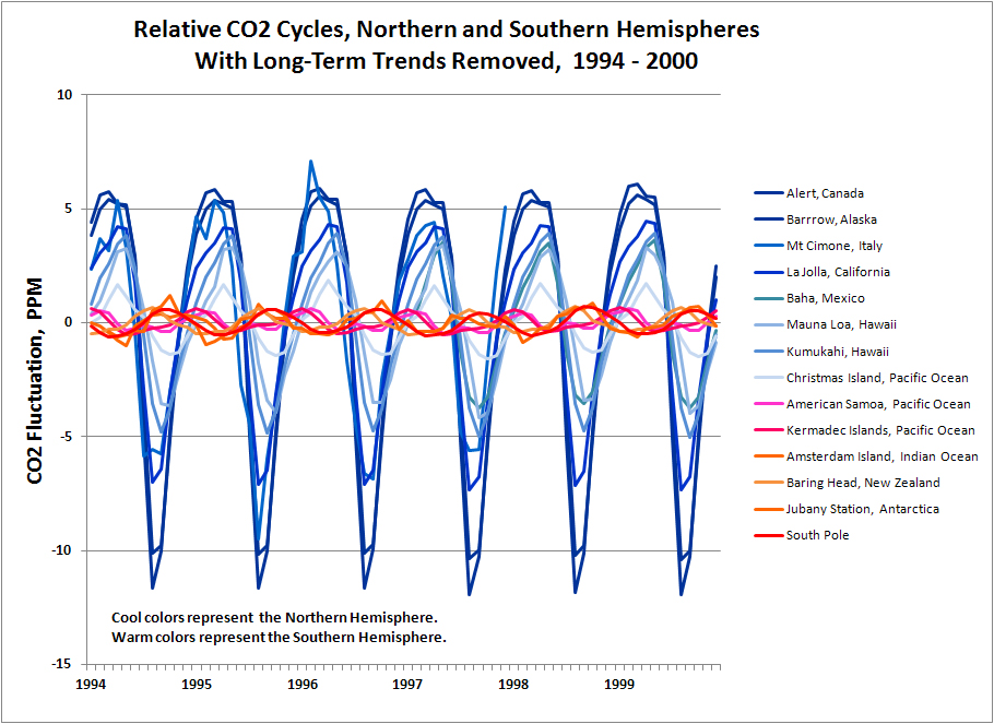
Figure 4. – Global Seasonal CO2 cycles with Long-term Trend Removed.

After removing the long-term trend from global CO2 observations, the remainder is the seasonal cycle.  A casual look at the chart reveals increasing amplitude of the cycle over the period of observations, particularly at high latitudes in the Northern Hemisphere. The amplitude can be extracted from the data, as shown in Figure 5.

Figure 5. – Amplitude of the Seasonal CO2 Cycle, Northern Hemisphere.

Amplitude of the seasonal CO2 cycle is growing.   If we add human population to the chart, we see a clear correlation between amplitude at high latitudes and human population.

Figure 8. – Amplitude of the Seasonal CO2 Cycle, Northern Hemisphere, with Global Population.

We can make a linear proportion between the amplitude of the seasonal cycle and population.  We can simply divide change in amplitude by the change in population, over the period of observations.   From that, we extrapolate that ratio to the point of zero population.   This gives us the portion of the seasonal cycle that is the result of human activities, and the remainder, which is the naturally occurring cycle..

The following table shows the fraction of the cycle amplitude which is due to human activities, and the fraction that is due to nature.

Fraction of Seasonal Cycle Amplitude
People Nature
                            Alert, Canada 30.2% 69.8%
                            Barrrow, Alaska                           37.8% 62.2%
                            La Jolla, California 74.0% 26.0%
                            Baha, Mexico                               30.8% 69.2%
                            Mauna Loa, Hawaii                       37.0% 63.0%
                            Kumukahi, Hawaii 34.5% 65.5%

The La Jolla data appears widely different from the other data, and was dropped from further calculations.  The average of the consistent observations shows that 34% of the 2009 seasonal cycle is the result of human activities, and 66% is the result of natural causes.

Made-Made CO2 Flux; Calculating Agriculture vs. Fossil Fuel Influence
Global agriculture produced 140 gigatonnes of biomass in 2009, removing about 96 gigatonnes of CO2 from the atmosphere.  Allocating agriculture by hemisphere by population gives a seasonal flux of 84.5 gigatonnes of CO2 in the Northern Hemisphere.

By contrast, total fossil fuel combustion produced 28.9 gigatonnes of CO2, substantially less than the seasonal CO2 flux due to agriculture.   And because fossil fuel use through the year is relatively consistent, data shows that there is only a 3.1 gigatonne seasonal flux of CO2 from fossil fuels in the Northern Hemisphere.   These figures show that 90 percent of the man-made portion of  the seasonal CO2 cycle is due to agriculture.

Calculating the Size of the Northern Hemisphere Biosphere
The relation established between amplitude of the seasonal cycle and volume of agricultural biomass, allows us to estimate the volume of natural biomass.   Ninety percent of the man-made amplitude change, or 30.6%, is due to agriculture, representing 140 gigatonnes of biomass, annually.   Natural forests, grasslands, and other seasonal growth in the Northern Hemisphere are responsible of 66% of the seasonal amplitude.  According to the volumetric relationship between seasonal amplitude and biomass established by agriculture, we can estimate the volume of plant growth in the temperate (seasonal) Northern Hemisphere.   The volume of natural, seasonal plants in the Northern Hemisphere is a little more the double the volume of agriculture, or 302 gigatonnes of biomass.  After corrections for carbon content, the natural seasonal volume in the Northern Hemisphere is 68 gigatonnes of carbon.

This estimate is based on the seasonal CO2 cycle of the Northern Hemisphere, and necessarily can only represent seasonal plant growth of the Northern Hemisphere.   All Southern Hemisphere biomass, equatorial oceans and rainforests, and non-seasonal biomass are excluded from the estimate.  But this finding may still be useful in modeling global the global CO2 cycle.

It is worth a quick comparison with other published estimates of the total global plant biomass.   Three respected sources include the U.S. Global Change Research Program, the U.S. Carbon Dioxide Information Analysis Center, and David McKay’s book, “Sustainable Energy Without the Hot Air”.
The US Global Change estimate for global vegetation biomass is 650 gigatonnes; the CDIAC estimate is 550 gigatonnes; and McKay’s cited estimate is 700 gigatonnes.

Our estimate of 300 gigatonnes for natural Northern Hemisphere seasonal biomass, plus 140 gigatonnes for agriculture yields 99 gigatonnes of carbon for seasonal growth in the Northern Hemisphere.  This appears to be reasonable, considering the range of estimates for global vegetation given above, including equitorial (non-seasonal) regions, the Southern Hemisphere, and the oceans.  If all estimates are correct,   Northern Hemisphere seasonal growth represents between 1/5 and 1/7 of total vegetation in the world

References:

Global CO2 concentration data in this report is credited to C. Keeling and others at the Scripps Institute of Oceanography, also Gaudry et al, Ciattaglia et al, Columbo and Santaguida, and Manning et al.  The data can be found on the Carbon Dioxide Information Analysis Center.

 http://cdiac.ornl.gov/trends/co2/

Data for CO2 released by fossil fuels is available from EIA CO2 Emissions from Fuel Consumption,
http://www.iea.org/co2highlights/co2highlights.pdf
And the BP Statistical Review of World Energy:
http://www.bp.com/sectionbodycopy.do?categoryId=7500&contentId=7068481

Global population figures from 1970 - 2010 were taken from Wikipedia.

The estimate for annual global agricultural biomass, circa 2009 was taken from a UN report:
http://www.unep.or.jp/Ietc/Publications/spc/WasteAgriculturalBiomassEST_Compendium.pdf

Monthly data for US fossil fuel consumption were taken from the EIA website:

http://www.eia.gov/

Estimates for global vegetation biomass were found on sites for the CDIAC, US Global Change Research Program, and David McKay's "Without the Hot Air".

http://cdiac.ornl.gov/pns/faq.html

http://www.climatescience.gov/Library/sap/sap2-2/final-report/

 This link is broken, but is the source for data used in this blog post.   It was a publication of the US Global Change Research Progam.

http://www.globalchange.gov/

http://withouthotair.com/

Global CO2 Summary -- The Keeling Curve, Seasonal CO2 Cycles, and Global CO2 Distribution

This blog post is a summary of several previous articles regarding atmospheric CO2.  This post consolidates and clarifies the previous posts.

Take a deep breath.   If you are about as old as me, that breath now contains about 25% more CO2 than your first breath when you were born, and about 42% more CO2 than when George Washington was president.  These numbers are changing rapidly, and have changed since I wrote my first post on this subject two years ago.

Abstract:

Atmospheric CO2 is rising globally, and has risen substantially in our lifetimes.  The CO2 content of the atmosphere is now higher than at any time in human history.    There is a seasonal cycle to CO2 concentration driven by growth and decay of plants in the Northern Hemisphere.  The CO2 cycle shows a strong fluctuation in the Northern Hemisphere and a very weak fluctuation of opposite polarity in the Southern Hemisphere.   Carbon isotopes show a similar global pattern of seasonal fluctuation and long-term change. 

A simple model can be constructed in an Excel spreadsheet using known volumes of agricultural production and fossil fuel consumption.  The model shows the global distribution of CO2, showing seasonal fluctuation and long-term increase identical to observed data.   The important thing is that the model was created using only data from human influences, although natural factors clearly exist and clearly affect atmospheric CO2.  The ease with which the model was generated, and the absence of quantifiable alternatives, clearly indicate that changes in atmospheric CO2 are primarily the result of human activities.

The Keeling Curve

The Keeling Curve is a set of CO2 measurements taken since 1958 on a mountaintop in Hawaii.  The measurements document seasonal CO2 change, and a long-term exponential rise in atmospheric CO2 concentration.   The Keeling curve at Mauna Loa fluctuates by about five ppm, peaking in the spring and reaching a minimum in the fall.  This week, the observatory announced that CO2 levels had exceeded 400 ppm for the first time at Mauna Loa. 

The Keeling Curve, as measured at Mauna Loa, has a seasonal cycle.  Atmospheric CO2 falls in the Northern Hemisphere summer, and rises during the Northern Hemisphere winter.  This is consistent with the absorption of CO2 by plants during the summer growing season, and the return of CO2 to the atmosphere through respiration or oxidation during the rest of the year.

Atmospheric CO2 has been measured at monitoring stations around the globe for a little over fifty years.

There is remarkable consistency of the long-term trend of CO2 across the globe, although details of the cycles differ.  The amplitude of the cycles varies dramatically by hemisphere and latitude.  The data on this chart are color-coded according to the monitoring stations shown above.

CO2 concentrations are rising everywhere on earth.   Superimposed on the rising curve is a cycle of seasonal fluctuation.  The fluctuation is strongest in the high latitudes of the Northern Hemisphere, and is weak in the Southern Hemisphere.  The following chart shows the seasonal CO2 cycle by latitude, with the long-term trend removed.

Long-Term CO2 Trends

Rising CO2 levels in the atmosphere are consistent with the volume of CO2 released by fossil fuels.  About 60%of the CO2 released by fossil fuels stays in the atmosphere; the remaining 40% is absorbed by earth systems acting as carbon reservoirs.  Examples include vegetation, the ocean, and precipitation of limestone.   We can compare the cumulative emissions to the observed change in atmospheric CO2, as seen in the following chart.

CO2 concentration in the Southern Hemisphere lags the rising concentration in the Northern Hemisphere.   The following chart shows the long-term trend at each CO2 monitoring station, with the seasonal cycle removed.

The average CO2 concentration in the Southern Hemisphere lags the Northern Hemisphere by about 2.7 ppm.  Looking at it another way, rising CO2 in the Southern Hemisphere lags the Northern Hemisphere by about 21 months.  

If we allocate fossil fuel emissions to each hemisphere by GDP, we see that 83% of CO2 emissions occur in the Northern Hemisphere.  Further, the 2.7 ppm difference in CO concentration between the hemispheres is a very close match to the annual excess CO2 emissions in the Northern Hemisphere.   The 21-month lag in the average CO2 level of the Southern Hemisphere represents the time required for atmospheric mixing of CO2 emitted in the Northern Hemisphere.

Pre-historic concentrations of CO2 are best known from air bubbles trapped in Antarctic ice.  Ice-cores have been recovered by drilling through the ice sheet.  The core was carefully dated by counting annual layers; by comparison with the deep-sea isotopic record; and by modeling the rate of ice accumulation.  Thousands of feet of core provide a continuous record going back 400,000 years.   Bubbles trapped in the ice are samples of the ancient atmosphere.   There is a small uncertainty regarding the time when the bubbles became permanently sealed, resulting in uncertainty of a few percent in the age of the trapped samples.   Current levels of atmospheric CO2, measured anywhere in the world, substantially exceed any sample recorded in ice cores for the past 400,000 to 800,000 years.

Pre-industrial levels of CO2 are estimated at about 280 ppm, based on ice-core data and a number  of 19^th century chemical analyses.    An exponential function can be fitted to the data, beginning with 281 ppm CO2 in the year 1800, and fitting the modern data of the Keeling curve.   Atmospheric CO2 is growing exponentially for the simple reason that human population and the use of fossil fuels are growing exponentially.  The exponential growth of fossil fuels use was well documented by geologist M. King Hubbert in his classic paper on peak oil, gas, and coal, published in 1955.

The exponential function allows prediction of future levels of atmospheric CO2.   A global average of 400 ppm (seen at Mauna Loa this month) is expected to be reached in 2015.   According to the forecast, 450 ppm will be reached in the year 2031, and 500 ppm in the year 2042.

The Seasonal CO2 Cycle
We see some interesting features when we look at the seasonal cycle closely.  Northern Hemisphere cycles are high amplitude, while the Southern Hemisphere is very low amplitude.  The expected polarity reversal only occurs in high Southern latitudes (near the pole).  Readings from latitudes less than 30 degrees south (near the equator; Kermadec Islands and American Samoa) share the polarity of the Northern Hemisphere.

The seasonal cycle has an amplitude of 17 ppm at high latitudes in the Northern Hemisphere, and diminishes toward the equator.  Amplitude of the cycle in the entire southern hemisphere is much lower, about 1 to 2 ppm.  The following chart shows the seasonal CO2 cycle with the long-term trend removed.

The amplitude of the CO2 cycle at high latitudes has increased since 1975 by about 3 ppm, from about 14 ppm to about 17 ppm.  The increasing magnitude of the seasonal cycle probably represents increasing human agricultural activity, as human population increased from about 3.5 billion in 1970, to over 7 billion today.

Global cyclicity is dominated by seasons in the Northern Hemisphere.  Polarity of the cycle in low latitudes (near the equator) of the Southern Hemisphere follows the seasonal patterns of the Northern Hemisphere.   Polarity of the seasonal cycle is reversed near the pole in the Southern Hemisphere.

The seasonality and asymmetry of the cycles is quite apparent.  In the Northern Hemisphere, CO2 falls sharply in the three months of summer, followed by an increase during the fall, winter and spring.  The increase is initially sharp in the fall, then more gradual through winter and spring.

Southern hemisphere cycles are low amplitude and symmetrical.  Polarity of the cycles at low latitudes (near the equator) follows the polarity of the Northern Hemisphere.

The obvious question is what drives seasonal CO2 cycles, and why the Northern Hemisphere is dramatically different than the Southern Hemisphere.  The Northern Hemisphere contains only two-thirds of the earths landmass, but 88% of the human population, and produces 83% of the worlds GDP.   We will explore these factors by modeling the CO2 cycle, considering both fossil fuel consumption and the photosynthesis/oxidation cycle, but first we should look at changes in carbon isotopes in the atmosphere.

Seasonal Carbon Isotope Cycles

Carbon mostly occurs in two naturally occurring isotopes: C12 and C13.   C12 comprises about 99 percent of carbon in the world, while C13 comprises most of the other percent.*  

The light isotope, C12, is more easily taken up in plants during photosynthesis. Coal and oil, which are derived from wood and algae, are enriched lighter isotopes.  The light isotope is also more easily metabolized by bacteria, which produce natural gas.  CO2 produced by burning fossil fuel reflects the carbon composition of the fuel, and is isotopically lighter than CO2 in the atmosphere.

The ratio of C13 to C12 is expressed as a standard measure: dC13/C12 (usually pronounced "del-thirteen").  The measure represents the ratio of C13 to C12, as compared to a standard ratio, in tenths of a percent.  The isotopic record for CO2 since 1970 shows a steadily declining value of dC13/C12, showing progressively lighter isotopic CO2 in the atmosphere.  

This long-term observed trend of isotopically lighter CO2 is consistent with an increasing contribution of fossil fuels to atmospheric CO2.  A simple calculation combining the isotopic composition of fossil fuels and the atmosphere would predict an even larger decline in atmospheric dC13/C12.   The modest decline observed in the data shows involvement of other carbon sinks in the environment, exchanging carbon with the atmosphere and moderating the dC13/C12 decline in the atmosphere.

Carbon isotopes show a seasonal fluctuation very similar to the CO2 seasonal cycle.   Strong seasonal fluctuation is observed in the Northern Hemisphere, and weak seasonal fluctuation in the Southern Hemisphere.  

The Northern Hemisphere, with much greater fertile land area than the Southern Hemisphere, removes a significant volume of light carbon from the atmosphere during the growing season.   The isotope cycle shows an asymmetry similar to the asymmetry of the CO2 cycle.  The isotopic composition of the atmosphere in the Northern Hemisphere rises sharply in the summer, and then declines gradually as a result of atmospheric mixing and oxidation of the biomass following the growing season.

Additional modeling of the carbon isotope data would be valuable.  We can make a back-of-the-envelope calculation of the expected change in atmospheric  dC13/C12 based on fossil fuel combustion.  The calculation shows a larger expected change than observed in the atmosphere.  We know that atmospheric CO2 is moderated by the action of various carbon sinks, which exchange carbon with the atmosphere.  Assuming an average fossil fuel dC13/C12 of -25, and the atmospheric dC13/C12 of -7.5 (1977), would suggest a decrease in atmospheric dC13/C12 to -9.5, a change of -2.0.   The actual decrease observed is only to -8.2, a change of -0.7.  This suggests that the volume of the total carbon reservoir actively exchanging carbon with the atmosphere is about twice the size of the total carbon in the atmosphere.    A more detailed model would provide greater confidence in this conclusion.

*C14, an unstable radioactive isotope, occurs in trace amounts in nature.  The radioactive isotope is important for age-dating anything containing carbon, within about 10 half-lives of the isotope, or about 60,000 years before present.  C14 was also produced by nuclear weapons but has been rapidly decreasing in the environment since the cessation of above-ground nuclear testing. 

Modeling Atmospheric CO2

A simple but quantitative model can be constructed to show the global distribution of atmospheric CO2, using an Excel spreadsheet.  Inputs to the model include agricultural biomass, fossil fuel emissions, absorption of excess CO2 by carbon sinks, and atmospheric mixing between the Northern and Southern Hemispheres.  The final model begins in the year 1971, and yields a set of CO2 curves by latitude that closely matches the actual record.

Model inputs include known quantities of fossil-fuel consumption over several decades and known volumes of agricultural biomass.  The model allocates fossil fuel emissions and agriculture by hemisphere (N & S), and applies a simple mixing model to yield CO2 concentration at five latitude positions on the earth.  The annual oxidation of agricultural biomass is inferred and modeled to fit observations of the CO2 cycle.

From earlier observations, the model was constructed using the following parameters:

• CO2 taken up by Plants during the growing season
• Oxidation  of carbon in plants following the growing season
• CO2 emissions from Fossil Fuels
• Absorption of CO2 by carbon sinks (e.g. oceans)
• Exchange of CO2 between Northern and Southern Hemispheres.

The CO2 seasonal cycle is dominated by the Northern Hemisphere, representing 67% of the earth's landmass, 90% of the human population (agriculture), and 83% of the industrial activity (GDP).  Modeling the cycle required consideration of fossil fuels and the photosynthesis/oxidation cycle.

Upon seeing the seasonal CO2 cycle in the Northern Hemisphere, my initial thought was that seasonal burning of fossil fuels accounted for much of the fluctuation.  Monthly consumption of oil, coal, and natural gas does show a seasonal fluctuation, with the correct polarity for the observed CO2 cycle.  However, fossil fuel consumption in the Northern Hemisphere produces only a 0.5 ppm seasonal cycle in atmospheric CO2, as compared to the 17 ppm cycle observed in actual data.  The following chart of seasonal CO2 emissions (with long-term growth of CO2 removed) was calculated from 2009-10 data from EIA and the BP Statistical Review of World Energy.  

The alternative consideration is that vegetation drives the seasonal CO2 cycle. In the summer, plants take up carbon through photosynthesis, and atmospheric CO2 declines.  Immediately following the growing season, plants give CO2 back to the atmosphere through oxidation, and CO2 rebounds sharply.

The model for seasonal CO2 uptake through photosynthesis was constructed beginning with the volume of biomass generated through agriculture.  Agriculture generates about 140 gigatonnes of biomass every year.
http://www.unep.or.jp/Ietc/Publications/spc/WasteAgriculturalBiomassEST_Compendium.pdf
After adjustments for the portion in the Northern Hemisphere (83%), moisture content (50%), carbon content (45%), and conversion to CO2 (3.67x) we can calculate about 96 gigatonnes of CO2 removed from the Northern Hemisphere atmosphere during the summer growing season.  Thus, during the growing season, CO2 in the Northern Hemisphere falls sharply.



The model distributed agricultural carbon and fossil fuel use according to economic output by hemisphere.  The Northern Hemisphere represents 83% of global economic output, and the Southern Hemisphere represents 17% of global economic output.
The following chart shows the monthly scheduling of photosynthesis, oxidation and fossil fuel consumption in the model for the Northern Hemisphere.

This model produced a surprisingly easy fit to the high latitude data of the Northern Hemisphere (see below).  There are no fossil fuel emissions in the model at this point, and the long-term trend of rising CO2 has been removed from the real-world data by subtracting an annual rolling average from the monthly data.

In modeling the Southern Hemisphere, I found that 17% of global agricultural biomass produced CO2 fluctuations that were far too large to match the data in the Southern Hemisphere. I found a good match by using only 5% of global agricultural biomass.   The chart below shows the model parameters.

Here is the modeled match to high-latitude Southern Hemisphere CO2, using 5% of global agricultural biomass.  It seems likely to me that the Southern Hemisphere photosynthesis/oxidation cycle is overwhelmed by CO2 mixing from the Northern Hemisphere, thus requiring a smaller volume to match the data.

A simple mixing model was generated to represent the cycles observed in intermediate latitudes.   The chart below shows a 50%-50% mixture at the equator, and 70% - 30% mixtures at intermediate latitudes.   As shown in the data above, the cycles of intermediate latitude (pink line) in the Southern Hemisphere follow the seasonal pattern of the Northern Hemisphere.

The final model runs from the year 1971 to 2009.  As a starting point, the model used values for the average CO2 concentration of the Northern and Southern Hemispheres in 1971, of 327 and 325 parts per million CO2, respectively.

The photosynthetic model, which was developed for the year 2009, was adjusted for earlier years as a function of global population. This resulted in cycles with increasing amplitude through the range of the model.  Agricultural production was assumed to vary directly as a function of population, but incremental agriculture was assumed to displace natural vegetation.  Growth of CO2 intake through photosynthesis was increased at a rate of 50% of incremental agricultural output (back-calculated from the 2009 model).

Although the fossil fuel input is much too small to account for the seasonal fluctuation in CO2, the long term effect is significant.  Carbon dioxide from fossil fuel emissions was added according to estimates from IEA and the BP statistical review of world energy.  Annual figures in these reports were scheduled on a monthly basis by analogy to US monthly consumption of coal, natural gas, and oil.  The volume of fossil fuel CO2 emissions was reduced by 40% to reflect the volume of CO2  absorbed by carbon sinks.

As previously noted, rising CO2 in the Southern Hemisphere lags CO2 in the Northern Hemisphere by a period of about 22 months.  The model was constructed to transfer half of the fossil fuel CO2 of the Northern Hemisphere to the Southern Hemisphere, using a lag of 22 months to represent the necessary mixing time.

Despite the general simplicity of the model, the resulting CO2 curve shows a reasonable correlation to actual data recorded across the global range of latitudes, and after 38 years of CO2 addition and subtraction, the model concludes at the appropriate concentrations of CO2 across the globe.

The most important conclusion from modeling global CO2 is that both long-term and seasonal change in atmospheric CO2 can be easily modeled using only inputs from human activities.
Other conclusions are as follows:

2)  Surprisingly, fossil fuel use does not have a significant effect on seasonal CO2 cycles.   Known volumes and timing of fossil-fuel emissions do not match the cyclicity in CO2 observations.

3)  Photosynthesis in the Northern Hemisphere dominates the seasonal CO2 cycle.  The model produced a good match to Northern Hemisphere seasonal CO2 using only agricultural biomass.  However, it is understood that natural biomass is also significant.  The agricultural volume is a proxy for the net volume of CO2 taken up and released by vegetation, in a more complex system.

 4)  Oxidation of vegetation occurs quickly.  Three quarters of the net seasonal biomass is oxidized in the first three months following the growing season.  Specifics on how and where this oxidation occurs would add confidence to the model.  Falling leaves and burning agricultural waste may account for some of the rapid oxidation following the growing season.

5)  The Northern Hemisphere dominates both seasonal and long-term trends in atmospheric CO2.  Global CO2 data and the model provide evidence for atmospheric mixing, to explain the 1) varying amplitude of seasonal CO2 cycles by latitude, 2) the lag of rising CO2 in the Southern Hemisphere, and 3) the gradation in phase of the cycles observed at intermediate latitudes.  The evidence of the degree and timing of atmospheric mixing may be useful in other areas of climate research.
6)  Calculations comparing isotope changes from fossil fuel emissions to the observed carbon isotope record suggest that the total reservoir of environmental carbon (including the atmosphere) is about three times the volume of carbon in the atmosphere.
------------
This post is a summary of previous posts about atmospheric CO2.  Additional details about the work can be found in these posts.

1)  The Keeling Curve

      http://dougrobbins.blogspot.com/2011/05/keeling-curve.html

2)  The Keeling Curve and Seasonal Carbon Cycles

      http://dougrobbins.blogspot.com/2012/03/keeling-curve-and-seasonal-carbon.html

3)   Seasonal Carbon Isotope Cycles

      http://dougrobbins.blogspot.com/2012/03/seasonal-carbon-isotope-cycles.html

4)   Long-Term Trends in Atmospheric CO2

      http://dougrobbins.blogspot.com/2012/03/long-term-trends-in-atmospheric-co2.html

5)   Modeling Global CO2 Cycles

      http://dougrobbins.blogspot.com/2012/04/modeling-global-co2-cycles.html

References:

Global CO2 concentration data in this report is credited to C. Keeling and others at the Scripps Institute of Oceanography, also Gaudry et al, Ciattaglia et al, Columbo and Santaguida, and Manning et al.  The data can be found on the Carbon Dioxide Information Analysis Center.

 http://cdiac.ornl.gov/trends/co2/

Data for CO2 released by fossil fuels is available from EIA CO2 Emissions from Fuel Consumption,
http://www.iea.org/co2highlights/co2highlights.pdf
And the BP Statistical Review of World Energy:
http://www.bp.com/sectionbodycopy.do?categoryId=7500&contentId=7068481

Monthly data for US fossil fuel consumption were taken from the EIA website:

http://www.eia.gov/

Global population figures from 1970 - 2010 were taken from Wikipedia.
The estimate for annual global biomass, circa 2009 was taken from a UN report:
http://www.unep.or.jp/Ietc/Publications/spc/WasteAgriculturalBiomassEST_Compendium.pdf

Source for ice-core data:  http://planetforlife.com/co2history/index.html

Modeling Global CO2 Cycles

This article is the fifth post in a series about Global CO2 trends and seasonal cycles.

1)  The Keeling Curve
      http://dougrobbins.blogspot.com/2011/05/keeling-curve.html

2)  The Keeling Curve and Seasonal Carbon Cycles

      http://dougrobbins.blogspot.com/2012/03/keeling-curve-and-seasonal-carbon.html

3)   Seasonal Carbon Isotope Cycles

      http://dougrobbins.blogspot.com/2012/03/seasonal-carbon-isotope-cycles.html

4)   Long-Term Trends in Atmospheric CO2

      http://dougrobbins.blogspot.com/2012/03/long-term-trends-in-atmospheric-co2.html

5)   Modeling Global CO2 Cycles

      http://dougrobbins.blogspot.com/2012/04/modeling-global-co2-cycles.html

In this post, I generate a model for the global CO2 record from 1971 - 2009.  Inputs to the model include agricultural biomass, fossil fuel emissions, absorption of excess CO2 by carbon sinks, and atmospheric mixing between the Northern and Southern Hemispheres.

The final model begins in the year 1971, and yields a set of CO2 curves, by latitude, that closely matches the actual record.

The important thing is that this model is made entirely by data resulting from human influences.   Natural factors also exist and clearly influence global CO2.  But the quantitative influence of agriculture and fossil fuel use is more than enough to model the annual cycles and long-term rise of CO2 in the atmosphere.

The ease with which the model was created, and the lack of any reasonable, quantifiable alternatives, indicate that changes in atmospheric CO2 are primarily the result of human activity.

Modeling

Modeling performs an important function in science.   After gathering data and making observations about pertinent parameters of a problem, it is necessary to put the pieces together in a quantitative model, to see if the parameters are acting as we expect.

The model “talks back” to us, in a way.   The model will show a fit to real-world data when our assumptions are reasonable, and a mis-fit to the data when the model is built on incorrect assumptions.   In this case, the model shows that the seasonal cyclicity of the Keeling curve is not the result of seasonal fossil fuel use, but instead is the result of seasonal photosynthesis and oxidation.  There is a good quantitative and geographic fit between the observed carbon cycles and the volume of carbon in agricultural biomass.   The increase of amplitude in CO2 cycles in proportion to population growth also supports the idea that the observed annual cycles are largely the result of agriculture.

This model considers separately the CO2 flux in the Northern Hemisphere and the Southern Hemisphere, and matches observations for the rate of mixing between the hemispheres.  A more complex model could be built, perhaps at increments of 5 or 10 degrees of latitude, and more closely identify the location of agriculture and fossil-fuel emissions, and that might be useful to addressing deeper questions.  But I believe a model should be simple in essence; sufficiently complex to answer the question at hand, and not any more complex.  This model is intended to answer the question of human influences on global CO2, and the division of the globe into two hemispheres is sufficient to answer that question.

Fossil Fuel Use and Annual Cycles

Fossil-fuel use has a cyclicity with the appropriate seasonal peaks for the Northern Hemisphere.  I spent quite a bit of time finding data on global fossil-fuel usage, assuming that it was a major factor in the Keeling curve annual cycles.  I extrapolated the seasonal patterns of use for coal, natural gas, and oil in the United States to global figures from the International Energy Agency (IEA) for the three commodities.  (I made an adjustment for the summer "air-conditioning"  bump in coal and natural gas, when extrapolating to the entire world.)

I converted the volumes (in gigatonnes) of CO2 emitted from fossil fuels to atmospheric CO2 concentrations in parts per million for the northern hemisphere and southern hemisphere.

In my last post,

http://dougrobbins.blogspot.com/2012/03/long-term-trends-in-atmospheric-co2.html, we saw that fossil fuel emissions are responsible for the long-term increase of atmospheric CO2.  But the peak of fossil fuel usage is in the months of December and January, but the steepest gains of CO2 occur in September through November.   In the fall months in high northern latitudes, CO2 concentrations rise by about 15 ppm.  The sum of fossil fuel emissions in those months total only about 1.5 ppm, an order of magnitude lower than the rise seen in the seasonal data.  Factors other than fossil fuels are causing most of the seasonal fluctuation of atmospheric CO2.

The Model

We can build a simple model to help identify the significant parameters driving global CO2 cycles, and quantify parameters wherever possible.   From our earlier observations, we can construct the model using the following parameters:

• CO2 taken up by Plants during the growing season
• Oxidation  of carbon in plants following the growing season
• CO2 emissions from Fossil Fuels
• Absorption of CO2 by carbon sinks (e.g. oceans)
• Exchange of CO2 between Northern and Southern Hemispheres.

 We already observed that the behavior of CO2 cycles differs greatly by latitude.  The Northern Hemisphere, with 68% of the world’s landmass, 88% of the world’s population, and 83% of the worlds GDP, has a cycle showing very large seasonal fluctuations in CO2.  The Southern Hemisphere shows much less annual CO2 fluctuation.  The sharpest and largest fluctuations in CO2 occur in the summer and fall months of the Northern Hemisphere.  In the summer, plants are taking up carbon through photosynthesis, and atmospheric CO2 declines.  Immediately following the growing season, CO2 concentration rebounds sharply, as plants give CO2 back to the atmosphere through oxidation.

I constructed a model for annual CO2 uptake through photosynthesis, beginning with the volume of biomass generated through agriculture.  Agriculture generates about 140 gigatonnes of biomass every year.
http://www.unep.or.jp/Ietc/Publications/spc/WasteAgriculturalBiomassEST_Compendium.pdf
Adjustments for moisture content (50%), carbon content (45%), and conversion to CO2 (3.67x) results in about 96 gigatonnes of CO2 removed from the Northern Hemisphere atmosphere annually.   Keep in mind that this is only half of the air on the planet.  Thus, during the growing season, CO2 in the Northern Hemisphere falls sharply.

In the model, I distributed agricultural carbon and fossil fuel use according to economic output by hemisphere.  The Northern Hemisphere represents 83% of global economic output, and the Southern Hemisphere represents 17% of global economic output.

I assigned the 96 gigatonnes of agricultural CO2 intake in the summer growing months, as shown in the following graph.  For the oxidation part of the cycle, we can observe a very sharp rebound in CO2 in the data during the fall months.  It is possible that some of the rebound is from CO2 sinks, seeking equilibrium after the change during the growing season.  However, isotope data shows an equally sharp rebound. (http://dougrobbins.blogspot.com/2012/03/seasonal-carbon-isotope-cycles.html)   It appears to me that vegetation is giving back to the atmosphere the very same CO2 that was absorbed during the summer.
I adopted an oxidation/respiration model to return the CO2 to the atmosphere as a zero-sum annual exchange.  I tried an exponential decline for the oxidation part of the cycle, then tweaked it to match the annual CO2 cycles of the Northern Hemisphere high latitudes (with the long-term trend removed).

This model produced a surprisingly easy fit to the high latitude data of the Northern Hemisphere (see below).
Note that the long-term rising CO2 trend has been removed from the real world data, and there are no CO2 emissions from fossil fuels in the model at this point.

The total volume of vegetation includes both natural as well as agricultural biomass.  I found a single estimate for the net global annual uptake by plants, of about 60 gigatonne of carbon, or about 220 gigatonnes of CO2.   According to these estimates, agriculture represents 52% of the total annual carbon uptake by plants.  Of the total annual carbon cycle, some carbon is exchanged with carbon sinks (soil) and some carbon exchanged with the atmosphere.  The fit of the model to observed data shows that the NET amount of carbon taken out of the atmosphere by plants, and returned by oxidation, is very close to the volume of carbon taken up by agricultural activity.

I followed a similar procedure to model the Southern Hemisphere.  I found that 17% of global agricultural biomass produced CO2 fluctuations that were far too large to match the data in the Southern Hemisphere. I found a good match by using only 5% of global agricultural biomass.   The chart below shows the model parameters.

The following chart shows the match of the model to the data from the Southern Hemisphere.

Annual cycles from intermediate latitudes have lower amplitude than cycles from the high northern latitudes.  This was the topic of an earlier post: http://dougrobbins.blogspot.com/2012/03/keeling-curve-and-seasonal-carbon.html.  The Northern Hemisphere, with its large CO2 fluctuations, dominates global CO2 cycles.  CO2 cycles from low latitudes in the Southern Hemisphere (pink) follow the seasonal pattern of the Northern Hemisphere, showing the range and influence of atmospheric mixing between Northern and Southern Hemispheres.

I tried a simple mixing model to represent the cycles observed in intermediate latitudes.   The chart below shows a 50%-50% mixture at the equator, and 70% - 30% mixtures at intermediate latitudes.   As shown in the data above, the cycles of intermediate latitude (pink line) in the Southern Hemisphere follow the seasonal pattern of the Northern Hemisphere.

A more sophisticated model could be created, using greater detail in the location of agriculture by latitude, but I think this model demonstrates that atmospheric mixing between the Northern and Southern Hemispheres can reasonably explain the range of amplitude in CO2 cycles in intermediate latitudes.

Global CO2 data show distinctive characteristics of annual cyclicity and a long-term rising trend ("the Keeling Curve").   Subtle aspects of the curve include a rising rate of increase, and an increase in the amplitude of the cycles.

The final model runs from the year 1971 to 2009.  As a starting point, the model used values for the average CO2 concentration of the Northern and Southern Hemispheres in 1971, of 327 and 325 parts per million CO2, respectively.

The photosynthetic model, which was developed for the year 2009, was adjusted for earlier years as a function of global population. This resulted in cycles with increasing amplitude through the range of the model.

Agricultural production was assumed to vary directly as a function of population, but incremental agriculture was assumed to displace natural vegetation.  Growth of CO2 intake through photosynthesis was increased at a rate of 50% of incremental agricultural output (back-calculated from the 2009 model).

Carbon dioxide from fossil fuel emissions was added, according to estimates from IEA and the BP statistical review of world energy.  Annual figures given in these reports were scheduled on a monthly basis, by analogy to US monthly consumption of coal, natural gas, and oil, as described above.  As noted in a previous post, about 40% of fossil fuel CO2 emissions are absorbed by carbon sinks, including the ocean.  This fraction of new carbon emissions was removed from the model on a monthly basis.

The Northern Hemisphere receives the bulk of fossil fuel CO2 emissions, and modeled CO2 rises rapidly in Northern Hemisphere, unless a transfer to the Southern Hemisphere is allowed.  In an earlier post, we saw that rising CO2 in the Southern Hemisphere lags CO2 in the Northern Hemisphere, by a period of about 22 months.  In the model, I transfered half of the excess CO2 of the Northern Hemisphere to the Southern Hemisphere, using a lag of 22 months to represent the necessary mixing time.

Despite the general simplicity of the model, the resulting CO2 curve shows a reasonable correlation to actual data recorded across the global range of latitudes, and after 38 years of CO2 addition and subtraction, the model concludes at the appropriate concentrations of CO2 across the globe.

Conclusions:

1)  A model can be generated which provides a very good match to the long-term global CO2 record.  The model includes estimated fossil fuel use, absorption of CO2 by carbon sinks, carbon accumulation in agricultural biomass, and oxidation of agricultural biomass.  The volume of agricultural biomass was varied in the model according to world population growth.

2)  Surprisingly, fossil fuel use does not have a significant effect on seasonal CO2 cycles.   Known volumes and timing of fossil-fuel emissions do not match the cyclicity in CO2 observations.

3)  Photosynthesis in the Northern Hemisphere, dominates the seasonal cycles.  The volume of CO2 absorbed through agriculture closely matches the net volume of CO2 taken up by both natural and agricultural photosynthesis.

 4)  Oxidation of vegetation occurs quickly.  Three quarters of the net plant biomass is oxidized in the first three months following the growing season.  It seems likely to me that burning of agricultural waste accounts for some of the rapid oxidation following the growing season.

5)  The Northern Hemisphere dominates both seasonal and long-term trends in atmospheric CO2.

6)  Mixing between the hemispheres accounts very well for the gradation of cyclicity observed at intermediate latitudes.

The model shows that the long-term trend of rising CO2 is attributable to fossil-fuel emissions.  Fossil fuel emissions account quantitatively for the rise in CO2 over the last 38 years, and fit the data with regard to differences in concentration in the Northern and Southern Hemispheres.
The model also shows that the annual cyclicity of the biologic cycle is strongly influenced by agriculture.  Agricultural biomass alone can be used to model  and match observed data for seasonal CO2 cyclicity.

And finally, the uptake of CO2 through agriculture clearly outpaces emissions of CO2 from fossil fuels, at least on a seasonal basis.  As a tool for the management of CO2 concentrations, policy-makers should consider banning the burning of agricultural waste, and consider options for disposal of agricultural waste as a means of sequestering significant volumes of carbon.
--------------
Global CO2 concentration data in this report is credited to C. Keeling and others at the Scripps Institute of Oceanography, also Gaudry et al, Ciattaglia et al, Columbo and Santaguida, and Manning et al.  The data can be found on the Carbon Dioxide Information Analysis Center.
 http://cdiac.ornl.gov/trends/co2/
Data for CO2 released by fossil fuels is available from EIA CO2 Emissions from Fuel Consumption,
http://www.iea.org/co2highlights/co2highlights.pdf
And the BP Statistical Review of World Energy:
http://www.bp.com/sectionbodycopy.do?categoryId=7500&contentId=7068481
Monthly data for US fossil fuel consumption were taken from the EIA website:

Global population figures from 1970 - 2010 were taken from Wikipedia.
The estimate for annual global biomass, circa 2009 was taken from a UN report:
http://www.unep.or.jp/Ietc/Publications/spc/WasteAgriculturalBiomassEST_Compendium.pdf