Rome Didn't Fall in A Day.


Objective Truth Exists and is Accessible to Everyone.

All Human Problems can be Solved with Enough Knowledge, Wealth, Social Cooperation and Time.


Photo: Rusty Peak, Anchorage, Alaska


Translate

Sunday, September 1, 2013

Consumption and the Road to A Sustainable Future


I saw an interesting video the other day.    The video is popularly known as “The Girl Who Silenced the World for Five Minutes”.   The speaker is Severn Suzuki.   At age 9, she founded the Childrens’ Environmental Organization (CEO), dedicated to learning and teaching other children about environmental issues.   In the video, at age 12, she is speaking at the International Earth Summit in Rio De Janeiro. 

The full text of her remarks (with a few errors) is found here:

Severn Suzuki, age 12, speaks about sharing.   

“In my country, we make so much waste.   We buy and throw away; buy and throw away; buy and throw away, and yet northern countries will not share with the needy.  Even when we have more than enough, we are afraid to share; we are afraid to let go of some of our wealth….
If a child on the streets, who has nothing, is willing to share, then why are we, who have everything, so greedy?....
I am only a child, yet I know that we are all in this together, and should act as one single world, towards one single goal….I am only a child, yet I know, if all of the money spent on war was spent on finding environmental answers, ending poverty, and finding treaties, what a wonderful world this would be.”

Suzuki’s comments address the two major social and economic problems of today’s world: The problem of relieving poverty, and the problem of environmental waste.   The problems are in part contradictory.  As economic development has raised standards of living across the world, consumption has increased.  As consumption increases, finite resources are depleted more quickly, and wastes accumulate. 

Why Do We Consume Wastefully?
Economist Thorstein Veblen (1857 – 1929) was an early graduate of Carleton College (yay, Carleton!) in Minnesota.   In his master work “Theory of the Leisure Class” Veblen coined the term “conspicuous consumption” – consumption solely for the purpose of demonstrating status in society.  A century ago, Veblen saw that this excess consumption leads to waste.  Today, our society has adopted wasteful practices for a variety of additional reasons: for convenience, to save time, and to enhance corporate profits.   

But as Velben noted, high rates of consumption lead to high levels of waste.  Higher consumption leads to faster depletion of resources.  As the standard of living increases around the globe, consumers change their habits, consuming more meat and processed foods, buying disposable products, and buying products which require more resources to produce and transport.  It is the reward of economic development, but carries environmental costs.

The Role of Sharing in the Global Economy
Sharing is a fundamental human gesture of kindness.  It is encapsulated in Karl Marx’s phrase: “From each according to his abilities, and to each according to his needs”, (once described to me as one of the highest expressions of human ethics). 

But sharing in modern economies and across international boundaries is complex.  Sharing goods without sharing employment provides no future.  Sharing employment (as in the low-wage factories of East Asia) without sharing wealth is exploitation.  Globalization and economic development of less-developed nations is a form of sharing, but must proceed according to decent standards of human rights, human dignity, worker safety, environmental responsibility and living wages, enforced by the purchasing practices of the companies importing goods from developing countries.  Companies buying goods in foreign markets have a responsibility to know their suppliers, and to buy from ethical manufacturers.  Consumers have a responsibility to know which products are produced ethically, and which are not, and to choose accordingly.

Awareness and oversight of working conditions in developing nations has improved over the past two decades, although there is clearly a long way to go.   Pressure from activists and consumers has forced companies such as Nike and Apple to evaluate the working conditions among their suppliers, and to improve the lives of those workers.  However, consideration of broader environmental issues has lagged behind the concern for workers’ rights.

Consumers buying a cheap pair of tennis shoes may consider the reputation of the brand with regard to workers’ rights, but rarely consider the environmental damage from the coal-fired electricity producing those shoes.   In sharing economic development with the less-developed world, the developed world has “over-shared” the environmental damage associated with development.  

In some cases, the environmental damage is literally exported to other countries.  In the mining of rare-earth elements, the United States formerly shipped raw ore to China, and Australia still ships ore to Malaysia for the separation of valuable metals from waste rock.  The waste rock (or tailings) from rare-earth mining is generally radioactive and highly toxic.  These wastes, of course, remain in the underdeveloped nation, while the valuable metal is returned to the developed nation in the form of products, leaving the environment of the developed nation pure and pristine, and the underdeveloped nation contaminated.

It seems that consumers and companies in the developed world need to be reminded of Severn Suzuki’s message:  “We are all in this together, and should act as one single world, toward one single goal.”

Paradoxes on the Path to a Sustainable Future
Industrialization has increased the standard of living in most countries on the globe.   Greater wealth is accompanied by many good things: better health care and education, increased life expectancy, decreased infant mortality and sustainable population growth.   Of these, the stabilization of population is perhaps the most important thing, as a requirement for a sustainable future.   But economic development also accelerates the depletion of resources, creates a growing gap between rich and poor, and degrades the environment.  This is particularly evident in China.

High rates of consumption require high production; high production requires rapid depletion of resources.  There is a conflict between the goal of industrialization for developing countries and the goal of decreasing the impact of production on the environment.  Economic development is necessary for the equality and dignity of the people in the developing world; but restraint is required to maintain environmental sustainability. 

Environmental writers, such as Donatello Meadows (principal author, Limits to Growth, the 30-Year Update) emphasize the need to reduce consumption to achieve sustainable levels of resource use.  However, consumption is the engine of modern economies.  The University of Michigan’s Consumer Confidence Survey is one of the most important indicators for the health of the American economy.  Lower rates of consumption may be driven by fear of economic or political instability, high interest rates or high energy prices.   When these conditions occur, low consumption inevitably pushes the economy into recession.  High unemployment and economic inefficiency are the result of widespread reductions in the rate of consumption.

So paradoxes and conflicts exist on the road to a sustainable future.  Environmental responsibility must be shared, along with wealth and economic development.  Consumption should be reduced to reduce the depletion of resources to sustainable levels, but developing nations must be allowed to improve the lives of their citizens, and to reap the rewards of economic development.   In some ways, this paradox requires restructuring of the economy, and of expectations in life.  Some of that restructuring has already been happening for the past 40 years.   As automation has replaced many workers in manufacturing, there has been a rise in the service sector of the economy.  Increasing numbers of workers are employed, not in manufacturing, but in providing services to their fellow human beings.  Perhaps this is the vision of a sustainable future:  a world in which we consume less, but in other ways to serve and care for our fellow man.
 -----
As an adult, Severn Cullis-Suzuki continues working as an environmental activist, organizer, speaker, and author.   She lives in British Columbia with her husband and two children.

Wednesday, August 14, 2013

Forecast of Carbon Dioxide Emissions and Atmospheric CO2

Global atmospheric CO2 is rising due to our use of fossil fuels.  This is the inescapable conclusion from freely available scientific data.   See my previous post on modeling global CO2 cycles:
http://dougrobbins.blogspot.com/2012/04/modeling-global-co2-cycles.html

The history of fossil-fuel CO2 emissions is well known from records of fossil-fuel sales.  Calculating the CO2 emitted by burning fossil fuels is simple, and we can compare global records of atmospheric CO2 to fossil-fuel emissions for the past 50 years.  About 60 percent of the CO2 emitted from fossil fuels remains in the atmosphere, and about 40 percent of the CO2 from fossil fuels is captured by carbon sinks, such as dissolution in the ocean or accumulation in soil.

The future of CO2 emissions and the consequent rise in atmospheric CO2  is the topic of this post.

History of CO2 Emissions
A study of fossil-fuel emissions was recently published by the CDIAC (Carbon Dioxide Information Analysis Center) – T.A. Boden, G. Marland, and R.J. Andres, 2013, Global, Regional, and National Fossil-Fuel CO2 Emissions, providing estimates of carbon dioxide emissions from 1751 – 2009.   To this data series, I added  estimates of future global carbon dioxide emissions for the years 2010 to 2040, published by the EIA (Energy Information Agency).  The figures presented are the EIA Reference Case, which is the base case of their forecast.  I extrapolated emissions from cement manufacture using a constant ratio to the fossil-fuel emissions, and eliminated emissions by flaring.

Here are the charts.
CO2 Emissions from 1751 to 2009.
The long-term chart follows the familiar exponential trend, first identified by M. King Hubbard in his landmark paper on peak oil in 1956.
The graph from 1900 to 2009 shows greater detail through the past century.
CO2 Emissions from 1900 to 2009.

Future CO2 Emissions
To the data series published by CDIAC, I added estimates for future global carbon dioxide emissions.   The U.S. Energy Information Agency (EIA) published projections of CO2 emissions for the years 2010 to 2040. The figures presented are the EIA Reference Case, which is the base case of their forecast (cases were also presented for high and low oil prices).  The charts show EIA estimates for various sources of emissions.  For consistency with the CDIAC data, I extrapolated emissions from cement manufacture using a constant ratio to the fossil-fuel emissions, and eliminated emissions by flaring.
CO2 Emissions History and Forecast, 1751 - 2040
In the EIA base case projection to 2040, the exponential increase of CO2 emissions is moderated, but CO2 emissions continue to increase.
CO2 Emissions and Forecast, 1900 - 2040

International Action to Reduce Fossil-Fuel CO2 Emissions
The rise of atmospheric CO2 was long suspected, but first documented in 1960 by Charles Keeling.   As evidence of global warming accumulated, a number of international conferences and treaties called for stabilizing or reducing CO2 emissions.  Beginning in 1988, The Intergovernmental Panel on Climate Change was formed.  A conference in Toronto during the same year recommended that by 2005, industrialized countries should reduce carbon emissions to 80% of the emissions levels of 1988.  Subsequent efforts include the UN Framework Convention on Climate Change (1992), the Kyoto Protocol of 1997, etc.

In concept, the Kyoto protocol calls for stabilizing global CO2 emissions at the 1990 level.   However, the Kyoto Protocol is a complex agreement, and actually only governs about one-quarter of the world’s carbon emissions as of 2010.  The United States never ratified the agreement.  Many other countries have no binding targets in the first period.   Japan and Russia, which observed binding targets in the first period, have declined to accept new targets in the second period.  Carbon Dioxide emissions for countries participating in the Kyoto Protocol actually fell 12% below 1990 levels by 2010.   But despite years of conferences and treaties, global CO2 emissions have continued to rise, and according to projections by the EIA, will continue to rise.

Future concentrations of Atmospheric CO2
Going from CO2 emitted by fossil-fuels to atmospheric CO2 requires a few calculations.   A simple volumetric calculation yields the concentration of CO2 released to the atmosphere; every 7.8171 Gigatonnes of CO2 emissions is equivalent to 1 ppm atmospheric CO2.   According to the experience of the last 50 years, only about 60% of the CO2 emissions remain in the atmosphere, so a corresponding reduction is made to forecast future atmospheric CO2 concentrations.

Historic CO2 levels are shown as a global average using a one-year rolling average from CO2 monitoring stations located from northern Canada to the South Pole.  Forecast CO2 concentrations were calculated according to the EIA forecast of CO2 emissions to 2040.  The chart of CO2 emissions and atmospheric CO2 is cumulative rather than annual, and is smoother than the charts of annual CO2 emissions.   Global average CO2 concentration is forecast to reach 450 ppm by the year 2032, and to reach 481 ppm by the end of the forecast period in 2040.
History and Forecast of Fossil-Fuel CO2 Emssions and Atmospheric CO2, 1970 - 2040

In summary, the base forecast for atmospheric CO2 is a continuation of the past trend.  Atmospheric CO2 will increase at an accelerating rate.  Future posts will address the recent effectiveness of renewable energy sources in reducing CO2 emissions, and limitations on the growth of renewable energy solutions.

The larger question is how humanity will deal with global warming which will result from higher concentrations of atmospheric carbon dioxide.  Strategies for coping include preventing the rise of atmospheric CO2; mitigating the effects of high CO2, or adapting to a warmer world.   A clear understanding of where we stand on these issues should help focus resources on the best solutions.
-----------------
References:
 T.A. Boden, G. Marland, and R.J. Andres, 2013, Global, Regional, and National Fossil-Fuel CO2 Emissions,  Carbon Dioxide Information Analysis Center

EIA 2013 Energy Outlook

EIA Forecasts

EIA Table Browser, interactive data-search tool
http://www.eia.gov/oiaf/aeo/tablebrowser

Institute for Energy Research; 2011 article and forecast.  In all cases, renewable energy represents only 14% to 17% of total energy supply.

Google data visualization; Globally, 4.7 tonnes of annual CO2 emissions per capita.

Tuesday, July 9, 2013

Methane Hydrates, in Deep Marine and Sub-Glacial Environments

Methane hydrate is a naturally occurring, unconventional source of natural gas.   Large volumes of potential gas resources exist in hydrate deposits in some deep-sea and arctic environments, but at the present time, technology for commercial production of methane hydrates does not exist.
Figure 1.   Burning methane hydrate.

Methane hydrate is a solid, crystalline form of methane and water, similar in appearance to ice.    Gas hydrates (also known as gas clathrates) are generally stable at temperatures below 40 degrees Fahrenheit and pressures higher than 1000 psi.  Hydrates are a familiar nuisance to petroleum engineers.   Hydrates will form in cold production flowlines, wherever temperature and pressure is conducive for the formation of hydrates.  Hydrates create flow obstructions or ice plugs; glycol anti-freeze is commonly injected for flow assurance.   

Gas hydrates, due to their solid, crystalline form, are very dense, concentrated forms of methane.   Gas hydrates contain 165 times more methane by volume than natural gas at surface pressure.  The volume of gas resource trapped in hydrates is large, but uncertain. 

Natural deposits of hydrates occur wherever natural gas and water meet at appropriate temperature and pressure.  This generally happens in deep water and within a few thousand feet of the surface in arctic environments.  Hydrates are found in the deepwater Gulf of Mexico, on the Blake Ridge offshore North Carolina, offshore West Africa, in the Sea of Japan, and in a variety of arctic petroleum basins, including the Alaskan North Slope.  

Japan is preparing to test an experimental offshore hydrate production well, using a production process tested in Canada in 2008 (Petroleum News, February 17, 2013).  Proposed production rates are minimal and only intended to demonstrate the technology.

Commercial production of gas hydrates was reported some years ago in a gas field in the Russian far north (IHS Energy).  Wells produce free gas from a reservoir below a gas hydrate cap.  As pressure in the reservoir declines, methane is released from the hydrates.   Gas recovery volumes are reported to indicate a contribution from the hydrate cap, but documentation is not available.

Deep Sea Gas Hydrates

The majority of known gas hydrate occurrences are in the deep ocean.  There, pressures and temperatures are favorable to the formation of hydrates.  Many gas hydrate sites are known from direct sampling at the sea-floor, or in shallow cores.  Hydrate sites are especially well-known in the Gulf of Mexico, where they occur over methane and petroleum seeps.  These seeps often occur in association with oil fields at depth, so they have necessarily been studied thoroughly in the course of exploration and development of oil fields in the Gulf of Mexico.  Chemosynthetic biological communities also frequently occur at petroleum seeps, and require surveys and protection from disturbance due to oil drilling. 

Gas hydrates are also known from seismic studies indicating the existence of hydrates.  The typical seismic indication is that of a “bottom-simulating reflector”, i.e., a seismic reflection parallel to the sea-floor, but not in conformance with the layering of the stratigraphy.   The bottom-simulating reflector represents the phase change from gas hydrate to water and gas, due to increasing temperature with depth.  The density change at the phase boundary is sufficient to cause an acoustic reflection.

Gas hydrates in the deep marine environment may serve as a seal for trapping oil and gas, or enhance the sealing capacity of an existing seal.   Such a trap might provide prospective potential very near the sea-floor.   On Blake Ridge offshore North Carolina, seismic studies indicate the likelihood of free gas below the gas hydrate, on a diapiric structure.  The gas hydrates near the sea floor probably enhanced the trapping characteristics of the diapir.

Figure 2.  Seismic displays indicating the probable existence of free gas trapped by gas hydrates on the Blake Ridge, offshore North Carolina (Taylor et al, 1999).

Gas Hydrates and Glaciation
The stability field of gas hydrates (low temperature, high-pressure) suggests an interesting possibility during recent geologic history.  Conditions favorable for the formation of hydrates must exist at the base of thick glacial ice.  During ice-age glaciation, conditions favorable for the formation of hydrates existed over large areas covered by continental ice sheets.  Where ice sheets covered gas-prone sedimentary basins, it seems inevitable that substantial volumes of hydrates would accumulate under the glacial ice.

Figure 3.   Methane Hydrate Stability Fields below glacial ice.    Gas hydrates will persist in the subsurface to a depth of about one kilometer below the ice.

Methane gas is normally produced in sedimentary basins, from both thermal alteration or biodegradation of organic matter (principally woody vegetation).   Methane rising naturally to the ground surface would be converted to gas hydrate near the base of the glacier.  Hydrates would accumulate over gas seeps throughout the period of the ice age, and would subsequently melt during deglaciation due to pressure release.   

Figure 4.   Petroleum Basin under continental ice sheets during the most recent glaciation.

Scientists exploring the sub-glacial lake Vostok in Antarctica expect gas hydrates to occur in or under the lake, due to the cold temperatures and high pressures present under four kilometers of ice.  Lake Vostok, a crescent-shaped rift lake, is a likely environment for the existence of petroleum source rock and thermally generated methane.   [Schematic diagrams showing hydrates invariably show the bulk of the hydrates at the bottom of the lake, for unknown reasons.  The bulk of the gas hydrate should be expected to be methane hydrate, which is lighter than water, and will rise to the top of the lake, at the base of the glacier. 
Figure 5.   Schematic of ice-core drilling on Lake Vostok, Antarctica.

During the most recent glacial period (about 100,000 years ago to 10,000 years ago), continental ice sheets covered a number of sedimentary petroleum basins, which were actively generating methane.  Where ice sheets covered these basins, gas hydrates would have been created.  When the ice melted, the gas hydrates would have disappeared; more from the loss of pressure than the change in temperature.   It is interesting to look at gas fields on the Alaska’s Kenai Peninsula, which may carry remnant signs of the former existence of hydrates.   Gas fields in this basin are often marked by low ground and wetlands immediately overlying the field (an observation pointed out to me by geologist Matt McCullough); and fields are marked by strong “gas chimney” seismic effects, due to large amounts of irreducible methane trapped in near-surface sediments.  Both of these features may reflect the previous existence of methane hydrates over the field.
Figure 6.  Area of Kenai Gas Field, Alaska, and overlying wetlands.

Risks of Gas Hydrate Production
Production of gas hydrate deposits carries the risk of depressurization and uncontrolled release of methane.  Once gas is released, it reduces the pressure on the hydrate reservoir, in a process similar to a geyser or a well blowout.   Such a depressurization, once initiated, might be impossible to stop.    Craters on the Blake Ridge indicate that a depressurization event occurred in the distant past, possibly releasing a volume of methane capable of affecting the global climate.
---------
References:


Methane Hydrates


Marine Hydrates
Marine Gas Hydrates and Their Global Distribution

Lake Vostok

Glaciation
Svendsen, J. et al., 2004, Late Quaternary ice sheet history of Eurasia. Quaternary Science Reviews, doi:10.1016/j.quascirev.2003.12.008)

Hydrostatic gradient  ==   981 kPascals per 100 meters


Friday, May 17, 2013

Global CO2 Summary -- The Keeling Curve, Seasonal CO2 Cycles, and Global CO2 Distribution


This blog post is a summary of several previous articles regarding atmospheric CO2.  This post consolidates and clarifies the previous posts.

Take a deep breath.   If you are about as old as me, that breath now contains about 25% more CO2 than your first breath when you were born, and about 42% more CO2 than when George Washington was president.  These numbers are changing rapidly, and have changed since I wrote my first post on this subject two years ago.

Abstract:
Atmospheric CO2 is rising globally, and has risen substantially in our lifetimes.  The CO2 content of the atmosphere is now higher than at any time in human history.    There is a seasonal cycle to CO2 concentration driven by growth and decay of plants in the Northern Hemisphere.  The CO2 cycle shows a strong fluctuation in the Northern Hemisphere and a very weak fluctuation of opposite polarity in the Southern Hemisphere.   Carbon isotopes show a similar global pattern of seasonal fluctuation and long-term change. 

A simple model can be constructed in an Excel spreadsheet using known volumes of agricultural production and fossil fuel consumption.  The model shows the global distribution of CO2, showing seasonal fluctuation and long-term increase identical to observed data.   The important thing is that the model was created using only data from human influences, although natural factors clearly exist and clearly affect atmospheric CO2.  The ease with which the model was generated, and the absence of quantifiable alternatives, clearly indicate that changes in atmospheric CO2 are primarily the result of human activities.

The Keeling Curve
The Keeling Curve is a set of CO2 measurements taken since 1958 on a mountaintop in Hawaii.  The measurements document seasonal CO2 change, and a long-term exponential rise in atmospheric CO2 concentration.   The Keeling curve at Mauna Loa fluctuates by about five ppm, peaking in the spring and reaching a minimum in the fall.  This week, the observatory announced that CO2 levels had exceeded 400 ppm for the first time at Mauna Loa. 
The Keeling Curve, as measured at Mauna Loa, has a seasonal cycle.  Atmospheric CO2 falls in the Northern Hemisphere summer, and rises during the Northern Hemisphere winter.  This is consistent with the absorption of CO2 by plants during the summer growing season, and the return of CO2 to the atmosphere through respiration or oxidation during the rest of the year.

Atmospheric CO2 has been measured at monitoring stations around the globe for a little over fifty years.
There is remarkable consistency of the long-term trend of CO2 across the globe, although details of the cycles differ.  The amplitude of the cycles varies dramatically by 
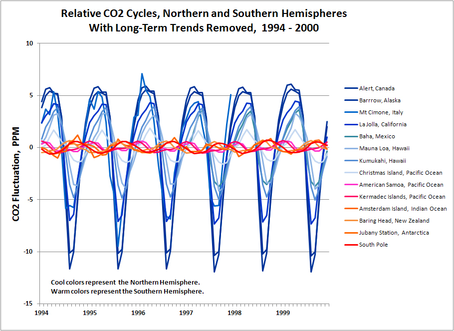
hemisphere and latitude.  The data on this chart are color-coded according to the monitoring stations shown above.

CO2 concentrations are rising everywhere on earth.   Superimposed on the rising curve is a cycle of seasonal fluctuation.  The fluctuation is strongest in the high latitudes of the Northern Hemisphere, and is weak in the Southern Hemisphere.  The following chart shows the seasonal CO2 cycle by latitude, with the long-term trend removed.

Long-Term CO2 Trends
Rising CO2 levels in the atmosphere are consistent with the volume of CO2 released by fossil fuels.  About 60%of the CO2 released by fossil fuels stays in the atmosphere; the remaining 40% is absorbed by earth systems acting as carbon reservoirs.  Examples include vegetation, the ocean, and precipitation of limestone.   We can compare the cumulative emissions to the observed change in atmospheric CO2, as seen in the following chart.
CO2 concentration in the Southern Hemisphere lags the rising concentration in the Northern Hemisphere.   The following chart shows the long-term trend at each CO2 monitoring station, with the seasonal cycle removed.


The average CO2 concentration in the Southern Hemisphere lags the Northern Hemisphere by about 2.7 ppm.  Looking at it another way, rising CO2 in the Southern Hemisphere lags the Northern Hemisphere by about 21 months.  
If we allocate fossil fuel emissions to each hemisphere by GDP, we see that 83% of CO2 emissions occur in the Northern Hemisphere.  Further, the 2.7 ppm difference in CO concentration between the hemispheres is a very close match to the annual excess CO2 emissions in the Northern Hemisphere.   The 21-month lag in the average CO2 level of the Southern Hemisphere represents the time required for atmospheric mixing of CO2 emitted in the Northern Hemisphere.

Pre-historic concentrations of CO2 are best known from air bubbles trapped in Antarctic ice.  Ice-cores have been recovered by drilling through the ice sheet.  The core was carefully dated by counting annual layers; by comparison with the deep-sea isotopic record; and by modeling the rate of ice accumulation.  Thousands of feet of core provide a continuous record going back 400,000 years.   Bubbles trapped in the ice are samples of the ancient atmosphere.   There is a small uncertainty regarding the time when the bubbles became permanently sealed, resulting in uncertainty of a few percent in the age of the trapped samples.   Current levels of atmospheric CO2, measured anywhere in the world, substantially exceed any sample recorded in ice cores for the past 400,000 to 800,000 years.
Pre-industrial levels of CO2 are estimated at about 280 ppm, based on ice-core data and a number  of 19th century chemical analyses.    An exponential function can be fitted to the data, beginning with 281 ppm CO2 in the year 1800, and fitting the modern data of the Keeling curve.   Atmospheric CO2 is growing exponentially for the simple reason that human population and the use of fossil fuels are growing exponentially.  The exponential growth of fossil fuels use was well documented by geologist M. King Hubbert in his classic paper on peak oil, gas, and coal, published in 1955.
The exponential function allows prediction of future levels of atmospheric CO2.   A global average of 400 ppm (seen at Mauna Loa this month) is expected to be reached in 2015.   According to the forecast, 450 ppm will be reached in the year 2031, and 500 ppm in the year 2042.
The Seasonal CO2 Cycle
We see some interesting features when we look at the seasonal cycle closely.  Northern Hemisphere cycles are high amplitude, while the Southern Hemisphere is very low amplitude.  The expected polarity reversal only occurs in high Southern latitudes (near the pole).  Readings from latitudes less than 30 degrees south (near the equator; Kermadec Islands and American Samoa) share the polarity of the Northern Hemisphere.

The seasonal cycle has an amplitude of 17 ppm at high latitudes in the Northern Hemisphere, and diminishes toward the equator.  Amplitude of the cycle in the entire southern hemisphere is much lower, about 1 to 2 ppm.  The following chart shows the seasonal CO2 cycle with the long-term trend removed.
The amplitude of the CO2 cycle at high latitudes has increased since 1975 by about 3 ppm, from about 14 ppm to about 17 ppm.  The increasing magnitude of the seasonal cycle probably represents increasing human agricultural activity, as human population increased from about 3.5 billion in 1970, to over 7 billion today.
Global cyclicity is dominated by seasons in the Northern Hemisphere.  Polarity of the cycle in low latitudes (near the equator) of the Southern Hemisphere follows the seasonal patterns of the Northern Hemisphere.   Polarity of the seasonal cycle is reversed near the pole in the Southern Hemisphere.

The seasonality and asymmetry of the cycles is quite apparent.  In the Northern Hemisphere, CO2 falls sharply in the three months of summer, followed by an increase during the fall, winter and spring.  The increase is initially sharp in the fall, then more gradual through winter and spring.

Southern hemisphere cycles are low amplitude and symmetrical.  Polarity of the cycles at low latitudes (near the equator) follows the polarity of the Northern Hemisphere.
The obvious question is what drives seasonal CO2 cycles, and why the Northern Hemisphere is dramatically different than the Southern Hemisphere.  The Northern Hemisphere contains only two-thirds of the earths landmass, but 88% of the human population, and produces 83% of the worlds GDP.   We will explore these factors by modeling the CO2 cycle, considering both fossil fuel consumption and the photosynthesis/oxidation cycle, but first we should look at changes in carbon isotopes in the atmosphere.

Seasonal Carbon Isotope Cycles
Carbon mostly occurs in two naturally occurring isotopes: C12 and C13.   C12 comprises about 99 percent of carbon in the world, while C13 comprises most of the other percent.*  

The light isotope, C12, is more easily taken up in plants during photosynthesis. Coal and oil, which are derived from wood and algae, are enriched lighter isotopes.  The light isotope is also more easily metabolized by bacteria, which produce natural gas.  CO2 produced by burning fossil fuel reflects the carbon composition of the fuel, and is isotopically lighter than CO2 in the atmosphere.

The ratio of C13 to C12 is expressed as a standard measure: dC13/C12 (usually pronounced "del-thirteen").  The measure represents the ratio of C13 to C12, as compared to a standard ratio, in tenths of a percent.  The isotopic record for CO2 since 1970 shows a steadily declining value of dC13/C12, showing progressively lighter isotopic CO2 in the atmosphere.  


This long-term observed trend of isotopically lighter CO2 is consistent with an increasing contribution of fossil fuels to atmospheric CO2.  A simple calculation combining the isotopic composition of fossil fuels and the atmosphere would predict an even larger decline in atmospheric dC13/C12.   The modest decline observed in the data shows involvement of other carbon sinks in the environment, exchanging carbon with the atmosphere and moderating the dC13/C12 decline in the atmosphere.

Carbon isotopes show a seasonal fluctuation very similar to the CO2 seasonal cycle.   Strong seasonal fluctuation is observed in the Northern Hemisphere, and weak seasonal fluctuation in the Southern Hemisphere.  

The Northern Hemisphere, with much greater fertile land area than the Southern Hemisphere, removes a significant volume of light carbon from the atmosphere during the growing season.   The isotope cycle shows an asymmetry similar to the asymmetry of the CO2 cycle.  The isotopic composition of the atmosphere in the Northern Hemisphere rises sharply in the summer, and then declines gradually as a result of atmospheric mixing and oxidation of the biomass following the growing season.
Additional modeling of the carbon isotope data would be valuable.  We can make a back-of-the-envelope calculation of the expected change in atmospheric  dC13/C12 based on fossil fuel combustion.  The calculation shows a larger expected change than observed in the atmosphere.  We know that atmospheric CO2 is moderated by the action of various carbon sinks, which exchange carbon with the atmosphere.  Assuming an average fossil fuel dC13/C12 of -25, and the atmospheric dC13/C12 of -7.5 (1977), would suggest a decrease in atmospheric dC13/C12 to -9.5, a change of -2.0.   The actual decrease observed is only to -8.2, a change of -0.7.  This suggests that the volume of the total carbon reservoir actively exchanging carbon with the atmosphere is about twice the size of the total carbon in the atmosphere.    A more detailed model would provide greater confidence in this conclusion.

*C14, an unstable radioactive isotope, occurs in trace amounts in nature.  The radioactive isotope is important for age-dating anything containing carbon, within about 10 half-lives of the isotope, or about 60,000 years before present.  C14 was also produced by nuclear weapons but has been rapidly decreasing in the environment since the cessation of above-ground nuclear testing. 

Modeling Atmospheric CO2
A simple but quantitative model can be constructed to show the global distribution of atmospheric CO2, using an Excel spreadsheet.  Inputs to the model include agricultural biomass, fossil fuel emissions, absorption of excess CO2 by carbon sinks, and atmospheric mixing between the Northern and Southern Hemispheres.  The final model begins in the year 1971, and yields a set of CO2 curves by latitude that closely matches the actual record.

Model inputs include known quantities of fossil-fuel consumption over several decades and known volumes of agricultural biomass.  The model allocates fossil fuel emissions and agriculture by hemisphere (N & S), and applies a simple mixing model to yield CO2 concentration at five latitude positions on the earth.  The annual oxidation of agricultural biomass is inferred and modeled to fit observations of the CO2 cycle.


From earlier observations, the model was constructed using the following parameters:
  • CO2 taken up by Plants during the growing season
  • Oxidation  of carbon in plants following the growing season
  • CO2 emissions from Fossil Fuels
  • Absorption of CO2 by carbon sinks (e.g. oceans)
  • Exchange of CO2 between Northern and Southern Hemispheres.

The CO2 seasonal cycle is dominated by the Northern Hemisphere, representing 67% of the earth's landmass, 90% of the human population (agriculture), and 83% of the industrial activity (GDP).  Modeling the cycle required consideration of fossil fuels and the photosynthesis/oxidation cycle.

Upon seeing the seasonal CO2 cycle in the Northern Hemisphere, my initial thought was that seasonal burning of fossil fuels accounted for much of the fluctuation.  Monthly consumption of oil, coal, and natural gas does show a seasonal fluctuation, with the correct polarity for the observed CO2 cycle.  However, fossil fuel consumption in the Northern Hemisphere produces only a 0.5 ppm seasonal cycle in atmospheric CO2, as compared to the 17 ppm cycle observed in actual data.  The following chart of seasonal CO2 emissions (with long-term growth of CO2 removed) was calculated from 2009-10 data from EIA and the BP Statistical Review of World Energy.  
The alternative consideration is that vegetation drives the seasonal CO2 cycle. In the summer, plants take up carbon through photosynthesis, and atmospheric CO2 declines.  Immediately following the growing season, plants give CO2 back to the atmosphere through oxidation, and CO2 rebounds sharply.

The model for seasonal CO2 uptake through photosynthesis was constructed beginning with the volume of biomass generated through agriculture.  Agriculture generates about 140 gigatonnes of biomass every year.
http://www.unep.or.jp/Ietc/Publications/spc/WasteAgriculturalBiomassEST_Compendium.pdf
After adjustments for the portion in the Northern Hemisphere (83%), moisture content (50%), carbon content (45%), and conversion to CO2 (3.67x) we can calculate about 96 gigatonnes of CO2 removed from the Northern Hemisphere atmosphere during the summer growing season.  Thus, during the growing season, CO2 in the Northern Hemisphere falls sharply.


The model distributed agricultural carbon and fossil fuel use according to economic output by hemisphere.  The Northern Hemisphere represents 83% of global economic output, and the Southern Hemisphere represents 17% of global economic output.
The following chart shows the monthly scheduling of photosynthesis, oxidation and fossil fuel consumption in the model for the Northern Hemisphere.


This model produced a surprisingly easy fit to the high latitude data of the Northern Hemisphere (see below).  There are no fossil fuel emissions in the model at this point, and the long-term trend of rising CO2 has been removed from the real-world data by subtracting an annual rolling average from the monthly data.

In modeling the Southern Hemisphere, I found that 17% of global agricultural biomass produced CO2 fluctuations that were far too large to match the data in the Southern Hemisphere. I found a good match by using only 5% of global agricultural biomass.   The chart below shows the model parameters.

Here is the modeled match to high-latitude Southern Hemisphere CO2, using 5% of global agricultural biomass.  It seems likely to me that the Southern Hemisphere photosynthesis/oxidation cycle is overwhelmed by CO2 mixing from the Northern Hemisphere, thus requiring a smaller volume to match the data.
A simple mixing model was generated to represent the cycles observed in intermediate latitudes.   The chart below shows a 50%-50% mixture at the equator, and 70% - 30% mixtures at intermediate latitudes.   As shown in the data above, the cycles of intermediate latitude (pink line) in the Southern Hemisphere follow the seasonal pattern of the Northern Hemisphere.
The final model runs from the year 1971 to 2009.  As a starting point, the model used values for the average CO2 concentration of the Northern and Southern Hemispheres in 1971, of 327 and 325 parts per million CO2, respectively.


The photosynthetic model, which was developed for the year 2009, was adjusted for earlier years as a function of global population. This resulted in cycles with increasing amplitude through the range of the model.  Agricultural production was assumed to vary directly as a function of population, but incremental agriculture was assumed to displace natural vegetation.  Growth of CO2 intake through photosynthesis was increased at a rate of 50% of incremental agricultural output (back-calculated from the 2009 model).


Although the fossil fuel input is much too small to account for the seasonal fluctuation in CO2, the long term effect is significant.  Carbon dioxide from fossil fuel emissions was added according to estimates from IEA and the BP statistical review of world energy.  Annual figures in these reports were scheduled on a monthly basis by analogy to US monthly consumption of coal, natural gas, and oil.  The volume of fossil fuel CO2 emissions was reduced by 40% to reflect the volume of CO2  absorbed by carbon sinks.

As previously noted, rising CO2 in the Southern Hemisphere lags CO2 in the Northern Hemisphere by a period of about 22 months.  The model was constructed to transfer half of the fossil fuel CO2 of the Northern Hemisphere to the Southern Hemisphere, using a lag of 22 months to represent the necessary mixing time.

Despite the general simplicity of the model, the resulting CO2 curve shows a reasonable correlation to actual data recorded across the global range of latitudes, and after 38 years of CO2 addition and subtraction, the model concludes at the appropriate concentrations of CO2 across the globe.

The most important conclusion from modeling global CO2 is that both long-term and seasonal change in atmospheric CO2 can be easily modeled using only inputs from human activities.
Other conclusions are as follows:

2)  Surprisingly, fossil fuel use does not have a significant effect on seasonal CO2 cycles.   Known volumes and timing of fossil-fuel emissions do not match the cyclicity in CO2 observations.
3)  Photosynthesis in the Northern Hemisphere dominates the seasonal CO2 cycle.  The model produced a good match to Northern Hemisphere seasonal CO2 using only agricultural biomass.  However, it is understood that natural biomass is also significant.  The agricultural volume is a proxy for the net volume of CO2 taken up and released by vegetation, in a more complex system.
 4)  Oxidation of vegetation occurs quickly.  Three quarters of the net seasonal biomass is oxidized in the first three months following the growing season.  Specifics on how and where this oxidation occurs would add confidence to the model.  Falling leaves and burning agricultural waste may account for some of the rapid oxidation following the growing season.
5)  The Northern Hemisphere dominates both seasonal and long-term trends in atmospheric CO2.  Global CO2 data and the model provide evidence for atmospheric mixing, to explain the 1) varying amplitude of seasonal CO2 cycles by latitude, 2) the lag of rising CO2 in the Southern Hemisphere, and 3) the gradation in phase of the cycles observed at intermediate latitudes.  The evidence of the degree and timing of atmospheric mixing may be useful in other areas of climate research.
6)  Calculations comparing isotope changes from fossil fuel emissions to the observed carbon isotope record suggest that the total reservoir of environmental carbon (including the atmosphere) is about three times the volume of carbon in the atmosphere.
------------
This post is a summary of previous posts about atmospheric CO2.  Additional details about the work can be found in these posts.

1)  The Keeling Curve
2)  The Keeling Curve and Seasonal Carbon Cycles
3)   Seasonal Carbon Isotope Cycles
4)   Long-Term Trends in Atmospheric CO2
5)   Modeling Global CO2 Cycles


References:


Global CO2 concentration data in this report is credited to C. Keeling and others at the Scripps Institute of Oceanography, also Gaudry et al, Ciattaglia et al, Columbo and Santaguida, and Manning et al.  The data can be found on the Carbon Dioxide Information Analysis Center.
Data for CO2 released by fossil fuels is available from EIA CO2 Emissions from Fuel Consumption,
http://www.iea.org/co2highlights/co2highlights.pdf
And the BP Statistical Review of World Energy:
http://www.bp.com/sectionbodycopy.do?categoryId=7500&contentId=7068481

Monthly data for US fossil fuel consumption were taken from the EIA website:


Global population figures from 1970 - 2010 were taken from Wikipedia.
The estimate for annual global biomass, circa 2009 was taken from a UN report:
http://www.unep.or.jp/Ietc/Publications/spc/WasteAgriculturalBiomassEST_Compendium.pdf